Next: Modelos de regressão Up: Análise de Sobrevivência Previous: Análise de Sobrevivência
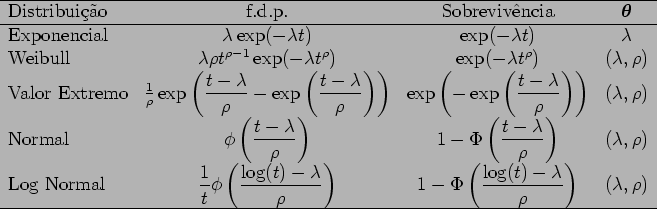
Assim para os modelos paramétricos temos na tabela ![]() a f.d.p e função de sobrevivência para algumas distribuições.
a f.d.p e função de sobrevivência para algumas distribuições.
Nos modelos paramétricos a função de sobrevivência e taxa de falhas dependem de um vetor de parâmetros
![]() que pode ser estimado via máxima verossimilhança, desta forma os estimadores de máxima verossimilhança para
que pode ser estimado via máxima verossimilhança, desta forma os estimadores de máxima verossimilhança para
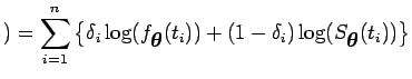
![]() são obtidos maximizando o log da verossimilhança dado abaixo
são obtidos maximizando o log da verossimilhança dado abaixo
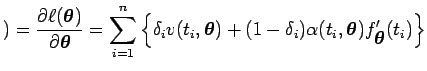
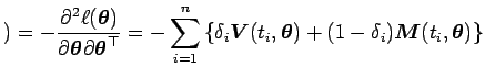
As derivadas parciais em relação a
![]() são
são
sendo
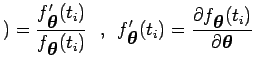
e

sendo que
![$\displaystyle )= \dfrac{\partial v(t_i,\mbox{\boldmath {$\theta$}})}{\partial \...
...mbox{\boldmath {$\theta$}}}(t_i)\right]}{\partial \mbox{\boldmath {$\theta$}}} $](img34.png)
Desta forma os estimadores de máxima verossimilhança são obtidos usando o algoritmo de Newton Raphson
Definimos
diag![]()
![]()
![]() como sendo uma matrix de zeros fora da diagonal principal e com os elementos de
como sendo uma matrix de zeros fora da diagonal principal e com os elementos de
![]() na diagonal principal. Assim, a convergência é obtida quando
na diagonal principal. Assim, a convergência é obtida quando
![]() é suficientemente pequeno. A estimação da função de sobrevivência e da função taxa de falhas é feita utilizando as propriedades de invariância dos estimadores de máxima verossimilhança, desta forma são dadas por
é suficientemente pequeno. A estimação da função de sobrevivência e da função taxa de falhas é feita utilizando as propriedades de invariância dos estimadores de máxima verossimilhança, desta forma são dadas por
Os testes de hipóteses do tipo
![]()
![]()
![]()
![]() contra
contra
![]()
![]()
![]()
![]() podem ser feitos via estatística de wald
podem ser feitos via estatística de wald
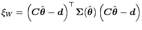
A distribuição assintótica de ![]() é uma
é uma ![]() , sendo
, sendo ![]() o posto da matrix
o posto da matrix
![]() .
.
A análise de resíduos pode ser feita utilizando o resíduo de Cox-Snell definido por
Se o modelo for adequado então
![]() . Assim poderíamos fazer gráficos quantil quantil dos resíduos de Cox-Snell contra uma distribuição
. Assim poderíamos fazer gráficos quantil quantil dos resíduos de Cox-Snell contra uma distribuição ![]() , caso os pontos do gráfico estejam próximos de uma reta com inclinação de aproximadamente 45 graus aceitamos o modelo proposto.
, caso os pontos do gráfico estejam próximos de uma reta com inclinação de aproximadamente 45 graus aceitamos o modelo proposto.