Basics of Probability Theory
In this lecture, we discuss the different meanings attributed to probability. We show how the Kolmogorov’s axioms of probability can be derived as a disposition to avoid sure loss. We then review the basic concepts of probability theory such as probability measures, random variables, conditional probability, joint probability distributions, independence, the total probability rule, the chain rule, and Bayes’ rule. We start with a historical account of the theory.
An unfinished gamble
The idea that one outcome is more probable than another outcome has long existed. However, it was not until the 17th century that a mathematical theory of uncertainty and randomness was developed. What started such rigorous study of the laws of uncertainty was the so-called problem of points, a somewhat frugal question on how to divide the stake of an unfinished gamble. By the end of the 15th century, some Italian mathematicians became interested in this problem without reaching a satisfactory solution. Then, in 1654, the problem was proposed to Pierre de Fermat and Blaise Pascal, who started a famous correspondence that would culminate in the first formalization of probability theory.1 The problem they discussed involved some unnecessary complications, but its essence can be put forward by the following example:
A gambling game between two players consists in tossing a coin repeatedly until one of the players accumulates 10 points. One player gets a point when the coin comes up heads, the other player gets a point when the coin comes up tails. Each player puts 50 Francs, making a pot worth of 100 Francs to be awarded to the winner. After playing a few rounds, one of the players is winning by 8 points to 7. Then, the game is suddenly interrupted to never be resumed. The question is: how should the players split the 100 Francs?
The solution proposed by Fermat and Pascal is rather trivial for anyone that has taken a basic course in probability theory, but was at the time very new: the stake should be divided in the same proportion as the number of cases that are favorable to each player, provided that each case is equally likely. Here is the rationale:
The key to the above solution is to consider only configurations with identical probabilities (whatever these might be). Had we simply listed the possible completions of the game (for example, that two heads straight ends the game in less than four tosses), that would have not been the case, as counting the number of favorable cases would produce an unfair split of the stake. Fermat’s ingenious solution was to break down the unequal probability scenarios into equal probability configurations. This procedure is at the heart of the principle of indifference (also called the principle of insufficient reason), which was proposed as a definition of probability nearly two centuries later by Pierre Laplace:
The theory of chance consists in reducing all the events of the same kind to a certain number of cases equally possible, that is to say, to such as we may be equally undecided about in regard to their existence, and in determining the number of cases favorable to the event whose probability is sought.
The principle of indifference can be understood as constructing uniform probabilities over spaces of elementary events that, when combined, form the events in which we are interested. According to Pascal and his followers, these elementary events should be assigned identical probability due to our inability of predicting the unique true event that will occur (or have occurred); this is an immediate conclusion of determinism, the belief that the occurrence of any event in nature can be precisely determined by the laws of mechanics if one possess sufficient knowledge (which is never the case).
What is probability
So what does it mean to say that “the probability of a fair die landing with number 4 up is 1/6” or that “the probability that the Amazon river is longer than the Nile river is 0.8”?
Classical probability
The classical interpretation of probability is to consider the probability of an event as the number of favorable cases divided by the total number of cases, where each case is considered equiprobable. This definition faces several shortcomings. First, taken literally, it is only applicable for a finite number of elementary events, so as to exclude probability over infinite domains. Second, it contains a circular character, as it presumes that probability has been defined for the elementary (equiprobable) events. Last, the probability of an event depends on the precise characterization of the elementary events, with different parametrizations leading to different probabilities.2 These difficulties encouraged mathematicians to seek for a non-epistemic interpretation.
Frequentist probability
The objectivist interpretation states that this number is a measure of the propensity of that event to naturally occur. In other words, by saying that the probability of a fair die landing 4 is 1/6 we are actually saying that if we (conceivably) roll the die infinitely many times, then at the limit 1/6th of rolls will end with the die landing with face 4 up. This interpretation views probability as a physical property of objects in the world, much in the same way as we see height, weight and distance. Unlike height, weight and distance, however, probabilities are assumed not be directly measurable; instead, they should be estimated from real observations. Probabilities need also to be agreed on by everyone, since they rely exclusively on the object and not on the observer. Objective probabilities thus need to be constrained only by the mathematical rules of relative frequencies (or proportions).
But what does it mean to say that the limiting relative frequency of an event (say, a coin landing heads up) is 1/2? The standard approach is to consider a sequence $a_1,a_2,\dotsc$, where each $a_i$ denotes the outcome of an experiment performed (ideally) under the exact same conditions (but oddly providing different results).3 Then, provided that this sequence converges, the frequentist probability of an event is taken to be
$$ \lim_{n \rightarrow \infty} \sum_i a_i/n \, . $$
While this definition appeals to intuition, it allows somewhat strange situations when seen from an operational viewpoint. For example, if the experiment is tossing a coin, and the first 100 tosses land heads up but all (infinitely many) tosses after that land tails, then the probability of heads is zero, irrespective of the fact that we have observed it occurring 100 times (of course, we would be dead after infinitely many observations). Also, the limiting frequency is sensitive to rearrangements of the sequence (e.g., compare a sequence of 0s and 1s, where a 1 follows a 0; with a rearrangement where each 1 is followed by 3 other 0s). Most importantly, the frequentist view disallows probabilities to be assigned to propositions that are elusive to repeating experimentation. Take for example the proposition ‘The Amazon river is longer than the Nile river’. A person might want to state that this proposition is true with probability 0.8; but the proposition is either true or false!.4 It is hard to imagine an experiment where the Amazon river will at times be longer than the Nile while at other times it will be shorter.
Subjective probability
Issues like these led de Finetti and many others to advocate a subjectivist interpretation of probability, by which the probability of an event is a measure of your belief about its occurrence. Probability thus expresses a personal state of knowledge. Under this view, events need not be repeatable, and different individuals might disagree on the probability of an event. In fact, instead of asking what is the probability of an event, one should instead ask for your probability. Subjective probabilities are measurable to the extent that an individual might be willing to disclose his or her intentions. Subjective probabilities are constrained by requirements of coherence, to assure that an individual will not hold conflicting or contradictory beliefs. This is usually derived by assuming that a rational agent should be disposed to act according to her beliefs. In short, your probability $P(A)$ specifies the value at which you are indifferent between accepting a gamble that either pays you $\$1$ if $A$ occurs and nothing otherwise, and surely receiving $P(A)$.
Axiomatic probability
The axiomatic interpretation views probability as an elementary concept, on which a formal theory is built and one that has no meaning per se. This is akin to the concept of a point in geometry. Probability theory, in this interpretation, should be concerned not with the nature of probability, but with consistency and completeness. Axioms might be inspired by the practice of probability (and statistics), but their validity should finally be decided by their ability to produce a system of well-formed and precise statements. The only constraints on probability values are those that enforce a consistent system, and those that allow us to assign probabilities to any object in the system. Within this view, the study of the laws of probability is a purely mathematical endeavor, much as the study of number theory. This view finds its place within the greater program of axiomatic mathematics, which has come to dominate the area.
The laws of probability
If probabilities are to be used to express knowledge and inform decisions (as is our general goal here), then it seems wise to investigate the consequences of an agent that acts according to the laws of probabilities. In fact, we can invert this reasoning and ask what should be such laws for an agent that displays some minimum desirable behavior. To this end, we will adopt the operational definition of probability, and declare that $P(A)$, the probability of an event $A$, is the fair price you are willing to pay for a ticket to a lottery that awards $\$1$ if event $A$ occurs and $0$ otherwise.5 An event is simply a set of states from the universe of discourse (which is as narrow or as wide as one so desires), and $\Omega$ is the sure event, which contains all states, also called the sample space.6 Since this price is declared fair, if I ask you to sell me the opportunity to take part in the lottery, you should be disposed to charge me the same price $P(A)$ you would pay for it.
If you so desire, you are allowed to equate $P(A)$ with the limiting relative frequency of a thought experiment, but in principle you are not forced to do so. In fact, your probabilities (or prices) for some event might differ from the probabilities of another person (as is usually the case when probabilities of complex events are elicited from pundits).
Fair prices and finitely additive probability
So what should we expect from your fair price? Since you can receive at most $\$1$, it is unreasonable to assign $P(A) > 1$ for any event $A$. And since your price is fair (that is, you should be willing to sell your ticket for the same price you are willing to buy it), your probability for an event that will certainly occur should be no less than $\$1$ (else you will certainly lose money selling the ticket). We thus have our first law of probability:
In a similar spirit, it would be meaningless to assign $P(A) < 0$. That would imply that you pay some amount to transfer the ticket to someone else, which is a worst scenario than simply setting $P(A) = 0$. We thus have our second law:
For the rest of this discussion it will be convenient to overload notation and equate an event $A$ with the $\{0,1\}$-valued function that returns $A(\omega)=1$ if $\omega \in A$, and $0$ otherwise. With this notation we can write that your net gain/loss from buying a ticket to the lottery related to event $A$ is $A(\omega)-P(A)$, which is a function from the unknown state of the world $\omega \in \Omega$. Similarly, your reward/loss for selling the ticket is $P(A) - A(\omega)$.
So consider disjoint events $A$ and $B$. Using our notation, we have that
$$
(A \cup B)(\omega) = A(\omega) + B(\omega)
$$
for all $\omega \in \Omega$. Now suppose you judge that $P(A \cup B) > P(A) + P(B)$.
Then if I buy tickets for lotteries $A$ and $B$ from you and sell you the ticket for lottery $A \cup B$, your overall net loss is
$$
\begin{multline*}
(A \cup B)(\omega) - P(A \cup B) + P(A) - A(\omega) + P(B) - B(\omega) = \\ P(A) + P(B) - P(A \cup B) < 0 \, ,
\end{multline*}
$$
whatever the state $\omega$ happens to be true. On the other hand, if you specify $$P(A \cup B) < P(A) + P(B)$$ then I can sell you tickets for $A$ and $B$ and buy your ticket for $A \cup B$, leaving you with a sure loss of $P(A \cup B) - P(A) - P(B)$.
Thus, to avoid losing money regardless of the state of the world (i.e., being a sure loser), you must specify your probabilities satisfying:
It turns out that those three rules are all the necessary requirements for avoiding sure loss.7 In particular, they are consistent with the properties of limiting frequencies; if
$$
P(A)= \lim_{n \rightarrow \infty} \sum_i a_i/n
\, \text{ and } \,
P(B)=\lim_{n \rightarrow \infty} \sum_i b_i/n \, ,
$$
and $A$ and $B$ are disjoint (so that $a_i + b_i \leq 1$), then
$P(A) \geq 0$, $P(B) \geq 0$, and
$$
\begin{align}
P(A \cup B) &= \lim_{n\rightarrow \infty} \sum_i (a_i + b_i)/n \\
&= \lim_{n \rightarrow \infty} \sum_i a_i/n + \lim_{n \rightarrow \infty}
\sum_i b_i/n \\
&= P(A) + P(B) \, .
\end{align}
$$
Also, if $a_i=1$ for every $i$ “large enough”, then $P(A)=1$, corresponding to the probability of the sure event.
Probability measure
We thus get to the standard definition of probability:
The set $\mathcal{F}$ can be any collection of events that you consider useful. When $\Omega$ is finite, there is no harm in assuming $\mathcal{F}$ to be the power set of $\Omega$, since any probability measure on $\mathcal{F}$ can be extended to the power set by application of Property \eqref{FA} (but you are not constrained to do so!). We will discuss what constraints need to be imposed on $\mathcal{F}$ for infinite sets later. It is customary to assume that $\mathcal{F}$ is a $\sigma$-algebra, meaning that it is closed under countable union of events. In that case, the triple $(\Omega,\mathcal{F},P)$ is called a probability space.
The following example helps consolidating the terminology and definitions discussed so far.
Let us revisit the problem of points. Recall that the first player gets a point when the coin lands heads (➊), and needs two points to win the game; the second player gains points when the coin lands tails (➋) and needs three points to win. The state space is $$ \Omega = \left\{ \begin{matrix} ➊➊➊➊, & ➊➊➋➊, & ➊➊➊➋, & ➊➊➋➋, \\ ➊➋➊➊, & ➊➋➋➊, & ➊➋➊➋, & ➊➋➋➋, \\ ➋➊➊➊, & ➋➊➋➊, & ➋➊➊➋, & ➋➊➋➋ , \\ ➋➋➊➊, & ➋➋➋➊, & ➋➋➊➋, & ➋➋➋➋ \\ \end{matrix} \right\} \, . $$ If you assume the coin is unbiased, then you should assign equal probabilities to the singleton events $\{ \omega \}$, for $\omega \in \Omega$ (otherwise you lose money by selling tickets for “underestimated” probabilities or by buying tickets for “overestimated” probabilities). Properties $\eqref{NN}$, \eqref{NU} and \eqref{FA} combined then imply that $P(\{ \omega \})=1/16$, coinciding with our initial informal analysis.
The event $A$ representing that the first player wins collects all states with at least two heads: $$ A = \left\{ \begin{matrix} ➊➊➊➊, & ➊➊➋➊, & ➊➊➊➋, \\ ➊➊➋➋, & ➊➋➊➊, & ➊➋➋➊, \\ ➊➋➊➋, & ➋➊➊➊, & ➋➊➋➊, \\ ➋➊➊➋, & ➋➋➊➊ \\ \end{matrix} \right\} \, . $$ Adding up the probabilities of each atomic (i.e., singleton) event, we get $$P(A) = 11/16 \, .$$ Call $B$ be the event that the second player wins. Since $A \cup B = \Omega$, it follows from $\eqref{NU}$ and $\eqref{FA}$ that $$ P(B) = 1 - P(A) = 5/16 \, . $$ As a consistency check note that the event that a heads is obtained in the third toss of the coin has probability $8/16=1/2$.
The previous formulation of the problem relates to LaPlaces’s principle of indifference. An alternative formulation that does not abide by that principle is to consider only the realizable completions of the game.
Consider again the problem of points, but now specify the state space as $$ \Omega = \left\{ \begin{matrix} ➊➊, & ➊➋➊, & ➊➋➋➊, \\ ➊➋➋➋, & ➋➊➊, & ➋➊➋➊, \\ ➋➊➋➋, & ➋➋➊➊, & ➋➋➊➋, \\ ➋➋➋ \end{matrix} \right\} $$ Still assuming that the coin is unbiased, we might assign the probability of each singleton proportional to the number of coin tosses: $P(\{ \omega \}) = 2^{-|\omega|}$, where $|\omega|$ denotes the number of symbols (coins) in state $\omega$. The probability of $B$ would in this case be given by $$ P(\{ ➊➋➋➋, ➋➊➋➋, ➋➋➊➋, ➋➋➋\}) = 3 \times 2^{-4} + 2^{-3} = 5/16 \, , $$ as before. Note that in this formulation events like the probability that the third coin lands heads is not 1/2 (in fact it is $P(\{➊➋➊,➋➊➊,➋➋➊➋,➋➋➊➊\})=3/8$), since some configurations of tosses are missing from the state space.
Countable additivity
Here is a more intricate example involving countably infinite events:
Consider a procedure (say, a computer program with access to a random number generator) which generates binary strings as follows: first a length $\ell > 0$ is generated with probability $1/2^\ell$, then a string of length $\ell$ is generated by tossing a fair coin $\ell$ times. The sure event is thus the countably infinite set $\Omega=\{0,1,00,01,10,11,001,\dotsc\}$. Let $\mathcal{F}$ denote the power set of $\Omega$; define your probability of observing a string $\omega$ as $$ P(\{\omega\}) = 2^{-2|\omega|} \text{ for } \omega \in \Omega \, , $$ where $|\omega|$ denotes the length of $\omega$. Since any event $A \in \mathcal{F}$ is countable, that is, it is either finite or countably finite, we can extend the above definition to any event $A$ by $$ P(A) = P\left( \bigcup_{\omega \in A} \{ \omega \} \right) = \sum_{\omega \in A} P(\{\omega\}) \, . $$ It is not difficult to see that this probability measure satisfies $\eqref{NN}$ and $\eqref{FA}$. For example, the probability that a string has length at most 3 is $$ \begin{align*} P(\{ \omega: |\omega| \leq 3\}) &= \sum_{i=1}^3 \sum_{\omega: |\omega|=i} P(\{\omega\}) \\ & = \sum_{i=1}^3 2^i 2^{-2i} = 2^{-1} + 2^{-2} + 2^{-3} = 7/8 \, . \end{align*} $$ To obtain $\eqref{NU}$ however we need a stronger property than finite additivity; we need that $$ P(\Omega) = \sum_{i=1}^\infty \sum_{\omega \in \Omega: |\omega|=i} P(\{\omega\}) = \sum_{i=1}^\infty 2^{-i}=1 \, . $$
The property that we required in the last example to derive $\eqref{NU}$ from the probability of basic events is called countable additivity.8 It is defined as follows.
Countable additivity is stronger than finite additivity in the sense that the former implies the latter but the converse is not true. Apart from ease of specification, is there any reason why we should assume a probability measure as countably additive? If we allow you to take part in an infinitely countable number of transactions (or lotteries), then one can show that countable additivity is both sufficient and necessary for avoiding sure loss. However, taking part in an infinite number of transactions removes the operational character of the behaviorist definition of probability. This reason lead de Finetti and many others to condemn countable additivity as a requirement for rationality (though you are still allowed to enforce it if you so desired). On the other hand, most measure-theoretic (i.e., axiomatic) approaches for probability theory assume countable additivity, and it is hard to find useful realistic examples which violate countable additivity. Curiously, countable additivity is not enforced by the properties of limiting relative frequencies. Countable additivity is also required for avoiding dynamic loss, that is, a situation where one infringes you a sure loss by combining your prices before and after the occurrence of some event.
Uncountably infinite states
In our previous examples, we have assumed that $\mathcal{F}$ is simply the power set of $\Omega$. For a countable number of states (assuming countable additivity), this is no restriction, as we can always extend the probability to the rest of the domain by enforcing \eqref{CA}. Is this also true for uncountable domains? To better motivate this question, consider the following example.
The simplest probability measure on an uncountable domain is arguably a uniform measure over the unit interval $\Omega=[0,1]$. By uniform, we mean that $$ P([a,b]) = b-a \, , $$ for $a \leq b$ (i.e., the length of the interval). The above equation includes the degenerate case of a singleton interval, since $$ P([a,a]) = P(a) = 0 \, . $$ This example shows that we cannot extend countable additivity to uncountable additivity, as that would imply that $P(\Omega) = \sum_{0 \leq x \leq 1} P(x) = 0$.9 Countable additivity, on the other hand, seems to work just fine, for example: $$ \begin{align*} P([a_1,b_1] \cup [a_2,b_2] \cup \dotsb) & = \sum_{i \in \mathbb{N}} P([a_i,b_i]) \\ & = \lim_{n \rightarrow \infty} \sum_{i=1}^n (b_i - a_i) \leq 1 \, , \end{align*} $$ for $$a_1 \leq b_1 \leq a_2 \leq b_2 \leq \dotsb $$ since $\cup_{i=1}^n [a_i,b_i] \subseteq \Omega$. So far so good, we can assign probabilities to intervals, and to countable unions of intervals. Can we extend $P$ to any subset $A$ of $\Omega$? One attempt at doing this is to consider coverings of $A$, that is, any countable collection of intervals $[a_1,b_1],[a_2,b_2],\dotsb$ (not necessarily disjoint), such that $A \subseteq \cup_i [a_i,b_i]$. Then we define the probability (or measure) of $A$ as $$ P(A) = \inf \left \{ \sum_i (b_i - a_i) : A \subseteq \cup_i [a_i,b_i] \right \} \, . $$
So the question is: is the quantity above well-defined for any $A$? The answer is negative: it can be show that there exists a collection of sets that cannot be assigned a probability measure altogether without producing some contradiction.
The impossibility of assigning a probability value to any subset of the unit interval is not a pathological case; this is true for any uncountable domain.
Thus, for uncountable domains, one needs to be careful to choose a domain $\mathcal{F}$. One typical choice is the so called Borel $\sigma$-algebra, which is formed by the countable unions and intersections of open sets. For example, the Borel $\sigma$-algebra on the reals $\mathcal{B}$ is the smallest $\sigma$-algebra that contains the (open) intervals (i.e., the sets $(a,b)$ for reals $a < b$). We will assume that $\mathcal{F}$ is this algebra when $\Omega$ is the real line, and denote it by $\mathcal{B}$. The elements of $\mathcal{B}$ are called Borel sets.
Conditional beliefs
Most often, we are interested in the probability of am event under the assumption that some other event is revealed. This sort of reasoning requires the use of conditional probabilities, which can be given an operational subjective interpretation in much the same way as unconditional probabilities, with the inclusion of the possibility of cancelling the lottery. Thus define $P(A|B)$ as your fair price for participating in a lottery that rewards you $\$1$ if events $A$ and $B $ occur and $\$0$ otherwise, and that is cancelled in case $B$ does not occur. By cancelled it is meant that you get the amount you paid back, and that you have to refund any buyer the exact amount paid. Hence, your net gain/loss for such a transaction is $B(\omega)[A(\omega)-P(A|B)]$. We can apply the same reasoning as before to conclude that your conditional belief should abide by rules $\eqref{NU}$, $\eqref{NN}$ and $\eqref{FA}$. In fact, your conditional probability is equivalent to your unconditional probability if we take $\Omega$ to be $B$. How should you set your conditional prices given your unconditional prices?
Your conditional and unconditional probability measures jointly avoid sure loss if and only if $$ P(A|B)P(B) = P(A \cap B) \, . $$
When $P(B) > 0$, the theorem above resorts to the usual axiomatic definition of conditional probability
$$ \begin{equation} \tag{CP} \label{CP} P(A|B) = \frac{P(A \cap B)}{P(B)} \, . \end{equation} $$
The above definition is usually justified as a re-normalization of your beliefs once an event is revealed. For $P(B)=0$, any price for $P(A|B)$ will suffice to avoid sure loss (but note that the traditional definition leaves the latter value undefined in this situation).
Random variables
The set-theoretic approach laid out is sufficient to describe simple scenarios like the examples given, but turns out to be cumbersome to represent more complex knowledge, involving many aspects of a domain or including numerical quantities such as counts, sums, etc. For instance, consider the case of the random string generation. To assign a probability to, say, the average length of a string, we can create a function $X$ that maps every string to its length. We can then query for example the probability that a string with length at most 5 is generated by $P(X \leq 5)=P(\{\omega \in \Omega: X(\omega) \leq 5\})$. The function $X$ thus defines a new probability space. A real-valued function on $\Omega$ such as $X$ is called a random variable.
The cumulative distribution function of a random variable $X$ is the real-valued function $F$ such that $$ F(x) = P(\{ \omega: X(\omega) \leq x \}) , \text{ for all real } x \, . $$
The standard definition of a random variable $X$ assumes that a probability space $(P,\Omega,\mathcal{F})$ is defined (and fixed), and requires that $F(x)$ be defined for any real $x$ (i.e., the set $\{ \omega: X(\omega) \leq x \}$ must be in $\mathcal{F}$). In practice, we usually specify the cumulative distribution function of the random variable, and implicitly consider an arbitrary probability space that generated it (there is always such a space), without caring to explicitly specifying it.
Probability distribution
The probability distribution of a random variable $X$ is the function $$ P_X(A) = P(\{ \omega: X(\omega) \in A\}) \, $$ defined on $\mathcal{B}$, the Borel $\sigma$-algebra of the reals. The triple $(\mathbb{R},P_X,\mathcal{B})$ is a valid probability space. We write $\Omega_X$ to denote the range of a variable $X$, that is, the set $\{ x: X(\omega) = x, \omega \in \Omega \}$. For convenience, we write $P_X(X = x)$ to denote the probability $P_X(\{ x \})$ of a singleton $\{ x \}$. Random variables are usually characterized by their distributions. Here are some commonly found random variables.
Given real values $a < b$, let $$ f(x) = \begin{cases} \frac{1}{b-a} & \text{if } a < x \leq b, \\ 0 & \text{otherwise}. \end{cases} $$ A uniform random variable has the distribution: $$ P(A) = \int_{A} f(x) dx \, , $$ whenever the integral exists.
The following example illustrate the use of uniform random variables and also a drawback of assining uniform distributions to represent ignorance.
Some liquid is made by composition of two other mixtures (such as water and wine, or gas and alcohol), and we are interested in assessing the relative quantities of each component. Suppose someone tells you that the liquid was prepared using 3 parts of one of the liquids to 1 part of the other, without specifying which is liquid is more abundant. Let $X$ be a random variable specifying the proportion of liquid A to liquid B, and $Y$ be a random variable specifying the proportion of liquid B to liquid A. The only information we have is that the relative proportion of liquids is in $[1/3, 3]$. Thus, a sensible strategy is to assume that both $X$ and $Y$ are distributed uniformly over the interval, that is, that $$ P_X(A) = P_Y(A) = \int_{A \cap [1/3,3]} \frac{1}{3-1/3} dx . $$ Now suppose you are interested in analysing the probability that $X \leq 2$. This is obtained as $$ P_X([1/3,2]) = (2-1/3)/(3-1/3) = 5/8 . $$ Similarly, we might be interesting is the probability that $Y \geq 1/2$. This is $$ P_Y([1/3,2]) = (3-1/2)/(3-1/3) = 5/(2*8) = 15/16 . $$ That is, even though both events $X \leq 2$ and $Y \geq 1/2$ are logically equivalent, the corresponding probabilities are different. This example demonstrates that probability functions are sensitive to the representation or encoding of the domain, and that the principle of indifference is ambiguous in that different representations lead to different specifications. It also suggests that assining uniform probabilities to represent ignorance is not necessarily uninformative (as it reflects our choice of representation).
Another very common distribution is the binomial distribution, which is usually motivated as the probability of observing $k$ heads in $n$ tosses of a coin.
Given parameters $\rho \in [0,1]$ and $n \in \mathbb{N}^+$, the binomial random variable has distribution $$ P(X = k) = {n \choose k} \rho^k(1-\rho)^{n-k} \, , $$ if $k \in \mathbb{N}$ and $P(X = k) = 0$ otherwise. The distribution can be extended to any Borel set by $\eqref{FA}$.
A very useful distribution distinguishes a single point:
An indicator random variable for a real value $x$ has the distribution:
$$
P(A) = \begin{cases}
1 & \text{ if } x \in A,\\
0 & \text{ if } x \not\in A,
\end{cases}
$$
for any measurable set $A$.
The Poisson random variable is commonly used to mode arrival in queuing theory:
Given a real-valued parameter $\lambda > 0$, the Poisson random variable has a distribution such that $$ P(X = k) = e^{-\lambda}\lambda^r/r! \, , $$ if $k \in \mathbb{N}$ and $P(X = k) = 0$ otherwise. The distribution can be extended to any Borel set by $\eqref{FA}$.
Discrete random variables
The support of a random variable is the set $\mathcal{D} \subset \mathbb{R}$ for which $P(\mathcal{D}) > 0$.
Random variables are categorized in terms of their support.
We say that a random variable is discrete if its support is countable. If the support is also finite, then the random variable is called simple or categorical.
If $X$ is a discrete random variable, then we can define its probability mass function:
The probability mass function $p$ of a random variable $X$ is the nonnegative function
$$p(x) = P_X(X = x) = P(\{ \omega: X(\omega) = x\})$$
for any $x$ in $\Omega_X$.
Discrete random variables are fully characterized by a probability mass function:
If $X$ is a discrete random variable with joint probability mass function $p$ then $$P_X(A) = \sum_{x \in A} p(x)$$ for every $A \subseteq \Omega_X$.
In practice, the result above allows us to specify a discrete random variable by specifying a probability mass function and assuming a consistent probability measure. Because of this, when discussing discrete random variables we often refer to a probability distribution or the probability mass functions interchangeably.
Functions of random variables
A function of a random variable is (usually) also a random variable. Thus, related random variables can be created as complex expressions of simpler variables. Consider the following example.
Let $X$ be a random variable such that $$ P(a \leq X \leq b) = \begin{cases} b - a , & \text{if } 0 \leq a < b \leq 1 \\ 0, & \text{otherwise}. \end{cases} $$ That is, $X$ follows a uniform distribution on the unit interval. Specify $$ Y = \lfloor 3X + 1 \rfloor \, . $$ Then, $Y$ has support/range $\{1,2,3\}$, and $P(Y=1)=P(Y=2)=P(Y=3)=1/3$.
The previous example shows that we can use a uniform distribution on the unit interval to create a uniform distribution over finitely many categories by simply composing random variables.
import random
def fairdice():
   x = random.random() # uniformly sample number in [0,1]
   y = int(6*x + 1)    # transformed variable
   return(y)
Here is a more intricate example of a random variable defined in terms of other random variables.
Suppose we are interested in the probability that exactly $k$ of the first $n$ bits of the binary representation of a number are equal to one. Define $P$ as the uniform probability measure on the unit interval
$\Omega=[0,1]$ such that $P([a,b]) = b-a$. Define $D_i$ as the random variable
returning the $i$-th bit in the infinite binary representation of a real-value $\omega$ in $\Omega$. That is,
$$\omega=\sum_{i \in \mathbb{N}} D_i(\omega)/2^i \, ,$$
where $D_i(\omega) \in \{0,1\}$.
For example, $D_1(\omega)=1$ if $\omega > 1/2$ and $D_1(\omega)=0$ if $\omega \leq 1/2$. Similarly, $D_2(\omega)=1$ if and only if $\omega \in (1/4,1/2] \cup (3/4,1]$. Each $D_i$ is a simple random variable with range/support $\{0,1\}$ and $p(D_i=0)=p(D_i=1)=1/2$. The latter follows from $\eqref{CA}$ since
$D_i$ partitions $\Omega$ in $2^i$ intervals of length (probability) $1/2^{i+1}$.
Let $S_n = \sum_{i=1}^n D_i$ be the sum of the first $n$ bits of a number in the unit interval.
Then $S_n$ is a binomial random variable with $\rho=1/2$:
$$p(S_n=k)={n \choose k} 2^{-n}$$
for $k \in \{0,\dotsc,n\}$.
The value returned by python function below follows the same distribution of $S_n$:
import random
def S(n):
    w = random.random() # sample number in [0,1]
    l, r  = 0.0, 1.0
    s = 0 # counts number of 1 bits in binary representation of w
    for _ in range(n):
      c = (l + r)/2
      if w > c:
        s += 1
        l = c
      else: r = c
    return(s)
Not every composition of random variables is a random variable due to the technicality that there must exist a probability space which “originates” it. However, composition of random variables not resulting in random variables are rare. In fact, arithmetic expressions (e.g., $2X^2 + 3Y/4 + 1$) and limits of random variables are always random variables.
Multivariate reasoning
Random variables are most useful when used in combination to specify a probabilistic model. This requires extending the concepts of distribution and other to collections of random variables.
The joint probability distribution of random variables $X_1,\dotsc,X_n$ is the function $$ P_{X_1,\dotsc,X_n}(A_1,\dotsc,A_n)=P(\{ \omega: X_i(\omega) \in A_i, i=1,\dotsc,n \}) \, , $$ defined on $\mathcal{B}^n$, the $n$-dimensional Borel $\sigma$-algebra.
We can also extend the concept of probability mass function:
If all random variables in $X$ are discrete, we define the joint probability mass function as $$ p(x_1,\dotsc,x_n) = P_{X_1,\dotsc,X_n}(X_1=x_1,\dotsc,X_n=x_n) \, . $$
The definitions above assume a fixed ordering for the variables. In practice, it is more convenient to consider a set of variables $X=\{X_1,\dotsc,X_n\}$ and to extend the definitions above so that they become invariant to permutations of the variables. For example, we can define the joint probability mass function of a set of discrete random variables $X$ as $$ p_X(\nu)=P(\{ \omega: X_i(\omega) = \nu(X_i), i=1,\dotsc,n \}) \, , $$ where $\nu$ is an assignment function, that maps each random variable $X_i$ in $X$ to a possible value $\nu(X_i)=x_i$. We abuse notation and write $$ P_X(X_1=x_1, \dotsc, X_n=x_n) = p_X(x_1,\dotsc,x_n) = p_X(\nu) \, , $$ thus effectively identifying a joint configuration $x_1,\dotsc,x_n$ with an assignment $\nu$.
Marginal probability
When working with a collection of random variables $X_1,\dotsc,X_n$, it is common to call a distribution $P_{X_i}$ of a single variable of a marginal distribution, and by extension the functions $F_{X_i}$ and $p_{X_1}$ their marginal cumulative and mass function distributions. Here is a very useful property concerning marginal and joint distributions:
If $X$ and $Y$ are random variables with marginal cumulative distributions $F_X$ and $F_Y$, respectively, and joint cumulative probability distribution $F_{XY}$, then: $$ F_X(x) = \lim_{y \rightarrow \infty} F_{XY}(x,y) \, . $$
Note the symmetry: the same result applies for the marginal of $Y$. A specialization of the above result for discrete random variables is very handy:
If $X$ and $Y$ are discrete random variables with marginal distributions $P_X$ and $P_Y$, respectively, and joint probability distribution $P_{XY}$, then: $$ P(X = x) = \sum_{y \in \Omega_Y} P(X = x, Y = y) \, . $$
The operation on the right hand side is called marginalization of the variable $Y$. The result can be extended to more than two random variables in a trivial way:
$$ P(X_1 = x_1) = \sum_{x_2 \in \Omega_{X_2}} \dotsb \sum_{x_n \in \Omega_{X_n}} P(X_1 = x_1, X_2 = x_2, \dotsc, X_n = x_n) \, . $$
Conditional probability distribution
Similarly to events, we can define the conditional probability distribution of a random variable $X$ given some event on random variable $Y$, written $P_{X|Y}( X \in A | Y \in B)$. As with conditional probability of events, this probability is only defined in $P(Y \in B)>0$, and must satisfy the identity
$$ P_{X|Y}(A | B)P_Y(B) = P_{XY}(A, B) \, . $$
Note that unlike the equation for events, the equation above considers three different probability measures $P_{X|Y}$, $P_Y$ and $P_{XY}$. We usually omit such subscripts, as the difference in measures can be inferred from the arguments; we also leave implicit the dependence on events, so for example, we might write the above identity as $$ P(X | Y) P(Y) = P(X, Y) \, . $$
We can extend marginalization to conditional distributions as well: $$ P(X = x| Z = z) = \sum_{y \in \Omega_Y} P(X = x, Y = y | Z = z) \, . $$ The equation above can be extended to several random variables in the trivial way.
The sinking of the Titanic is the deadliest maritime disaster of the twentieth century. The table below displays the counts of survivors and deceased according to sex and class.
| Gender | Class | Status | Total | Joint Probability |
|---|---|---|---|---|
| male | 1 | deceased | 118 | 0.195 |
| male | 1 | survived | 57 | 0.09 |
| male | 2 | deceased | 154 | 0.255 |
| male | 2 | survived | 14 | 0.023 |
| female | 1 | deceased | 4 | 0.006 |
| female | 1 | survived | 146 | 0.24 |
| female | 2 | deceased | 13 | 0.021 |
| female | 2 | survived | 104 | 0.17 |
The last column is obtained by renormalizing the counts (i.e., dividing by their sum), and specifies a joint probability mass function over categorical random variables $G$, $C$ and $S$, representing gender, class and status, respectively. Assume $G=1$ denotes male, $G=2$ denotes female, $S=1$ denotes deceased and $S=2$ denotes survived. By applying the definition of conditional probability, we find that $$ P(S = 2 | G = 1, C = 1) = \frac{P(S = 2, G = 1, C = 1)}{P(G = 1, C = 1)} \, . $$ The denominator can be obtained as the marginal of the joint distribution: $$ P(G=1, C=1) = P(S = 1, G = 1, C = 1) + P(S = 2, G = 1, C = 1) = 0.285 \, . $$ Thus, $P(S = 2 | G = 1, C = 1) \approx 0.32$. Repeating this procedure for the other conditioning events, we obtain the following table of marginal conditional probabilities of survival $P(S=2|G=g, C=c)$.
| Gender | Class | Marginal Conditional Probability |
|---|---|---|
| male | 1 | 0.32 |
| male | 2 | 0.07 |
| female | 1 | 0.976 |
| female | 2 | 0.89 |
Note the algorithmic procedure. Each row of the table above is obtained by renormalizing the corresponding rows in the first table, so that their sum equals one. For example, the first row is obtained by renormalizing the first two rows of the first table to make the corresponding probabilities add up to one. This is performed by dividing by their sum, $0.195 + 0.09 = 0.285$, which is exactly the same as dividing by $P(G=1, C=1)$.
Bayes’ rule
Conditional probabilities satisfy several other properties with respect to other conditional and unconditional probabilities. Arguably the most famous of these properties is Bayes’ rule, which follows by simple arithmetic manipulation of the above equation.
If $A$ and $B$ are such that $P_X(A) > 0$ and $P_Y(B) > 0$, then $$ P_{X|Y}(A| B) = \frac{P_{Y|X}(B|A)P_X(A)}{P_Y(B)} \, . $$
These rules can be extended to more than two variables, for example:
For any random variables $X$, $Y$ and $Z$ we have that $$ P(X| Y, Z) = \frac{P(Y|X, Z)P(X | Z)}{P(Y | Z)} \, , $$ whenever the conditional probabilities are defined.
Note that we have used the simplified notation where subscripts are dropped and the arguments are represented by the corresponding random variables.
Even though the Bayes’ rule establishes a relation between the conditional and unconditional probability of a variable, these two quantities can represent very different and contradictory beliefs, as the next example shows.
While the effects of the COVID-19 pandemics have been felt worldwide, its consequences have differed significantly from country to country. While such difference can be attributed to varying factors such as the countries income, the response strategy, and even political views, the age population profile seems to be a major influence for case fatality rate (i.e., the proportion of deaths among confirmed cases). The table below shows official data from case fatality rates (in %) in Italy and China, according to Age groups.10
| Age | 0-9 | 10-19 | 20-29 | 30-39 | 40-49 | 50-59 | 60-69 | 70-79 | 80+ | Total |
|---|---|---|---|---|---|---|---|---|---|---|
| Italy | 0 | 0 | 0 | 0 | 0.1 | 0.2 | 2.5 | 6.4 | 13.2 | 4.3 |
| China | 0 | 0.2 | 0.2 | 0.2 | 0.4 | 1.3 | 3.6 | 8 | 14.8 | 2.3 |
The last column marginalizes the age and reports the case fatality rates for the entire population.
Let $D=1$ denote a fatality, $A$ denote an age group and $C$ the country. According to the table, we have that $$ P(D=1|A=a,C=\text{Italy}) < P(D=1|A=a,C=\text{China}) $$ for all age groups $a$, even though $$ P(D=1|C=\text{Italy}) > P(D=1|C=\text{China}) \, , $$ according to the last column. This reversal in trend when shifting from an unconditional to a conditional probability is referred to as Simpson’s Paradox. Despite its name, there is no paradox here. This type of relation between conditional and unconditional probabilities does not violate any of the laws of probabilities that we discussed. The confusion arises when one ascribes a causal meaning to the event, a meaning which probabilities per se do not convey.
The chain rule
A property at the heart of the theory of probabilistic graphical models is the so-called Chain Rule, which allows us to write a joint distribution as a product of marginal conditional distributions:
For any set of random variables $X_1,\dotsc,X_n$ it follows that $$ P(X_1,\dotsc,X_n) = P(X_1)P(X_2|X_1) \dotsb P(X_n|X_1,\dotsc,X_{n-1}) \, . $$
We say that the right-hand side of the equation above is a factorization of the probability on the left-hand side, just like $2 \times 3$ is a factorization of $6$. Note that the ordering/indexing of the variables is arbitrary. In fact, the property holds for any permutation of the indices. A simple arithmetic manipulation shows that the property is true for conditional distribution on the left-hand side: $$ P(X_1,\dotsc,X_n | Y) = P(X_1 | Y)P(X_2|X_1, Y) \dotsb P(X_n|X_1,\dotsc,X_{n-1}, Y) \, . $$
Independence
Independence is actually an extra-mathematical and qualitative notion, one of utmost importance for the practice of probabilistic modeling. In fact, most of this course is focused on creating a language to describe independence assertions. Intuitively, a set of independent random variables is such that knowing the state of any subset of the variables brings no information to any other subset of variables. Formally:
Random variables $X_1,\dotsc,X_n$ are unconditionally independent if their joint distribution factorizes as the product of their marginals: $$ P_{X_1,\dotsc,X_n}(A_1,\dotsc,A_n) = P_{X_1}(A_1)P_{X_2}(A_2) \dotsb P_{X_n}(A_n) $$ for any combination of measurable sets $A_{1},\dotsc,A_{n} \subseteq \mathbb{R}$.
Using our simplified notation, we can rewrite the above condition as $$ P(X_1,\dotsc,X_n) = \prod_{i=1}^n P(X_i) \, . $$
If $X$ and $Y$ are random variables such that $P(X, Y) > 0$ (hence $P(X) > 0$ and $P(Y) > 0$), it follows that $P(X|Y)=P(X)$ if and only if $X$ and $Y$ are independent. This connects the definition above with our intuitive notion of independence as irrelevance of knowledge. This property can be extended to any number of variables.
We can also define independence in terms of conditional probabilities:
Random variables $X_1,\dotsc,X_n$ are conditionally independent given random variable $Z$ if $$ P(X_1,\dotsc,X_n | Z) = \prod_{i=1}^n P(X_i | Z) \, . $$
Note that conditional independence and independence are unrelated properties: one can occur without the other. Another important thing to notice is that independence of a subset of random variables does not imply independence of a larger subset. These facts are shown by the next example.
Consider an experiment where two fair coins are tossed; if either they both with heads up or both with heads down a third coin is placed tails up, otherwise, the third coin is placed heads up. Thus let $X$, $Y$ and $Z$ be the outcomes of the first, second and third coin, respectively, with 1 denoting heads and 0 denoting tails. Then $P(X=x)=P(Y=y)=P(Z=z)=1/2$. Knowing the result of one of the coins gives no information about another coin: $$ P(X|Y) = P(Y|X) = P(X|Z) = P(Z|X) = P(Y|Z) = P(Z|Y) = 1/2 \, . $$ That is, any two pair of variables are unconditionally independent. Yet, the third coin is a deterministic function of the first two coins thus $$ P(Z = 1| X = 1, Y = 1) = 0 \, . $$ Therefore, even though the variables are pairwise independent, they are not all three independent. Moreover, $X$ and $Y$ are not independent given $Z$: $$ P(X = 1, Y = 1 | Z = 1) = \frac{P(Z = 1 | X = 1, Y = 1)P(X = 1, Y = 1)}{P(Z=1)} = 0 \, , $$ which differs from $$ P(X=1|Z=1)P(Y=1|Z=1) = 1/4 \, . $$
The following example combines several of the concepts seen so far.
Suppose we are interested in finding the probability that all the persons in a group of $n \leq 365$ persons will be born in a different day of the year. Fix an ordering of the persons, and let $B_1$ denote the birthday of the first person, $B_2$ the birthday of the second person, and so on. These random variables are independent: $$ P(B1,\dotsc,B_n) = \prod_{i=1}^n P(B_i) = \left( \frac{1}{365} \right)^n \, . $$ We are interested in the probability that all variables take on different values. Thus define $D$ as a random variable that takes on value 1 if all birthdays are different and 0 otherwise. We want therefore to compute $$ \begin{align*} P(D=1) &= \sum_{b_1} \sum_{b_2} \dotsb \sum_{b_n} P(Z=1,B_1=b_1,\dotsc,B_n=b_n) \\ & = \sum_{b_1} \sum_{b_2} \dotsb \sum_{b_n} \prod_{i=1}^n P(B_i=b_i) P(D=1|B_1=b_1,\dotsc,B_n=b_n) \, . \end{align*} $$ Notice that we can move the probability $P(B_1,\dotsc,B_n)$ outside the sums as they are constant with respect to the values of these variables, obtaining: $$ P(D=1) = \frac{1}{365^n} \sum_{b_1} \dotsb \sum_{b_n} P(D=1| B_1=b_1,\dotsc,B_n=b_n ) \, . $$ We can now work out the sums from right to left. For $i=1,\dotsc,n-1$, define $$ \psi_i(b_1,\dotsc,b_i) = \begin{cases} 1 & \text{if } b_i \neq b_j \text{ for } i \neq j, \\ 0 & \text{otherwise}. \end{cases} $$ Then $$ \sum_{b_n} P(D=1| b_1,\dotsc,b_n ) = (366-n)\psi_{n-1}(b_1,\dotsc,b_{n-1}) \, , $$ as there are $365-(n-1)$ values for $B_n$ that differ from a given configuration $b_1,\dotsc,b_{n-1}$ such that all values are different. Similarly $$ \sum_{b_{n-1}} \psi_{n-1}(b_1,\dotsc,b_{n-1}) = (367-n)\psi_{n-2}(b_1,\dotsc,b_{n-2})\, . $$ The final formula is $$ P(D=1) = \frac{1}{365^n}\prod_{i=1}^n(366-i) = \frac{365!}{365^n(365-n)!} \, . $$ For $n=23$, this value is roughly $0.493$.
Here is another important example of the use of the concepts we have seen.
The Monty Hall Problem is based on an old US TV game show, and spurred a lot of controversy when it was revived as a brain teaser in a popular magazine. The problem is as follows. The game show hosted by Monty Hall (hence the name) consisted of a participant selecting one of three doors available. One of the doors hides a hefty prize (say, a brand new car ownership), while the other two doors hide goats. After the participant makes a selection, the host opens one of the remaining doors hiding the goats, and gives the participant the possibility of switching to the other door. The problem consists in decided whether changing doors is beneficial to the participant.
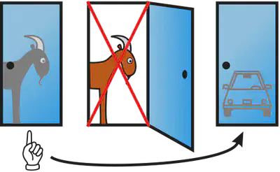
Assume that doors are numbered 1,2,3 and let $C$ be a random variable representing the location of the car prize, $S$ a random variable representing the door selected by the participant and $R$ the ensuing door revealed by the host. The key step to the solution of the problem is to realize that the revealed door bears a logic constraint with respect to the doors selected by the participant and the door hiding the car prize, as the host always reveals a door hiding a goat, so that it is not selected at random. We assume that the location of the car is selected uniformly at random, thus $P(C = i)=1/3$ for $i = 1, 2, 3$. Consider a situation where the participant selects door $j$ and the hosts reveals door $k \neq j$. The solution resides in deciding whether $$ P(C = i | S = j, R = k) > P(C = j | S = j, R = k) \text{ for } i \neq j,k \, . $$ That is, the participant should switch to door $i$ if and only if it has greater probability of hiding the car prize than its current selection $j$. To compute such probabilities, we apply the conditional Bayes’ rule: $$ \begin{align*} P(C = i | S = j, R = k) &= \frac{P(R = k | C = i, S = j)P(C = i | S = j)}{P(R = k | S= j)} \\ & = \frac{P(R = k | C = i, S = j)P(C = i | S = j)}{\sum_{c=1}^3 P(R = k | C = c, S = j)P(C = c | S = j)} \, . \end{align*} $$ Concerning the numerator, note that when the participant selects a door not containing the car (i.e., $i \neq j$) the host has only one possible door to reveal, thus $P(R = k | S = j, C = i) = 1$. As for the denominator, note that when the participant selects the door containing the car, we assume that the host selects arbitrarily between any of the remaining doors, therefore $P(R = k | S = j, C = j) = 1/2$. Also, the host never reveals the door hiding the car, hence $P(R = k | S = j, C = k) = 0$. Finally, the location of the car is not affected by the selection of the participant (and vice-versa), so that $P(C = c|S = i)=P(C = c)=1/3$. In other words, $S$ and $C$ are (pairwise) independent. We thus find that $$ P(C = i | S = j, R = k) = 2/3 > 1/3 = P(C = j | S = j, R = k) \, . $$ Hence, on average, the participant is better off switching doors (irrespective of the initial selection and the revealed door).11
Continuous random variables
We can also consider random variables with uncountably infinite support.
We say that a random variable $X$ is continuous if there is a nonnegative (Lebesgue) integrable function $f$ such that $$ P(a \leq X \leq b) = \int_a^b f(x) dx \, , $$ for any reals $a \leq b$.
The definition above implies that $P(X = x) = P(x \leq X \leq x) = 0$ for any value $x$, thus coinciding with our intuition of a continuous random quantity. The function $f$ is called the probability density function of $X$, or more simply, the density of $X$. Note that we allow $f$ to be discontinuous at a finite number of points (e.g., $f$ can be piecewise continuous) with probability zero. By construction, if $F$ is the cumulative distribution of $X$ then $F(x)=\int_{-\infty}^x f(u) du$. By the Fundamental Theorem of Calculus, if $F$ is differentiable then
Given real-valued parameters $\mu \in \mathbb{R}$ and $\sigma > 0$, we define a Gaussian random variable as having the distribution $$ P(A) = \int_{A} \frac{1}{\sigma\sqrt{2\pi}}\exp\left( - \frac{(x-\mu)^2}{2\sigma^2} \right) dx \, , $$ for any set $A$ for which the integral exists.
Here is a common continuous random variable used for modeling arrival of items:
Given a real-valued parameter $\lambda > 0$, let $$ f(x) = \lambda e^{-\lambda x} , $$ if $x \geq 0$ and $f(x) = 0$ otherwise. The Exponential Distribution is defined as $$ P(A) = \int_{A} f(x) dx , $$ whenever the integral exists.
A probability density function can take values larger than one. The Gaussian random variable has a density function that is larger than unity for certain values of $\sigma$. Here’s another example of a density function whose maximum is greater than 1:
Continuity of the cumulative distribution function does not suffice to ensure that a random variable is continuous, as there are continuous probability distributions which are zero except on a set of Lebesgue measure zero, yet each point in that set has probability zero (hence the distribution is also not discrete).12 The converse however is true: if $X$ has a continuous density then its cumulative function is continuous.
We can extend the concepts of multivariate reasoning for collections of continuous random variables. For example:
If $X_1,\dotsc,X_n$ are continuous random variables, we define their joint probability density function as the function $f(x_1,\dotsc,x_n)$ such that $$ P(\{\omega: X_i(\omega) \in A_i\}) = \int_{A_1} \dotsb \int_{A_n} f(x_1,\dotsc,x_n) dx_1 \dotsb dx_n \, , $$ whenever that integral exists.
We have defined a conditional distribution $P( X \in A | Y \in B)$ under the assumption that $P(Y \in B)>0$. This works well for discrete random variables, but is unsatisfactory for continuous random variables; often we want to model a phenomenon assuming an observation; if the random variable being assumed observed is continuous, then $B=\{y\}$ will be a singleton with probability zero. We could instead assume that $B$ is in fact an infinitesimal region around the observation $y$, one large enough to have positive probability: $$ P(X \in A | Y = y) = \lim_{\Delta \rightarrow 0} P(X \in A| Y \in [y-\Delta/2,y+\Delta/2]) \, . $$
The World Pool-Billiard Association specifies two standard sizes of pool tables with playing surface lengths of 254cm and 234cm. Suppose you have one such table and you perform the following experiment. You throw a billiard ball $n$ times from a initial arbitrary position and with enough force so that the ball bounces multiples times until it reaches a resting position. You assume that the distance $X$ of the resting position to the left edge of the table is distributed uniformly. Assuming that either length is equally probable, what is the distribution of the length $L$ of the table given $n$ measurements?
First note that if any of the measurements is above 234 and bellow 254, then the probability of $L=234$ is zero. Thus let us assume that all $n$ measurements are below 234.13
Consider an interval $B(x) = [x - \Delta/2, x + \Delta/2]$ for each measurement $x$. Since measurements are assumed uniformly distributed, the likelihood of observing a set-valued measurement $B(x)$ given that the table length is $L$ is $$ P(X \in B(x) | L) = \int_{B(x)} \frac{1}{L} dx = \Delta/L \, . $$
By Bayes’rule, the posterior probability that the length is 234cm given the interval-valued measurements is $$ \begin{align*} P(L = 234 & \mid X_1 \in B(x_1), \ldots, X_n \in B(x_n)) \\ & = \frac{\prod_{i=1}^n P(X_i \in B(x_i) \mid L = 234)P(L=234)}{\sum_{l \in \{234,254\}} \prod_{i=1}^n P(X_i \in B(x_i) \mid L=l)P(L=l)} \\ & = \frac{(\Delta/234)^n(1/2)}{ (\Delta/234)^n(1/2) + (\Delta/254)^n(1/2)} = \frac{254^n}{234^n+254^n} \, . \end{align*} $$ Note that the value above does not depend on the interval length $\Delta$. Hence, $$ \begin{align*} P(L=234|X_1=x_1,\dotsc,X_n=x_n) &= \lim_{\Delta \rightarrow 0} P(L \mid X_1 \in B(x_1), \ldots, X_n \in B(x_n)) \\ &= \frac{254^n}{234^n+254^n} = \frac{1}{1 + (234/254)^n} \, . \end{align*} $$ The same value could be reached by considering the conditional density of a measurement $X$ given the table $L$: $$ \begin{align*} f_X(x | L=k) &= \frac{d F_X(x)}{dx} \\ & = \lim_{\Delta \rightarrow 0} \frac{1}{\Delta} (P(X \leq x + \Delta/2 | L) - P(X \leq x - \Delta/2 | L)) \\ & = \frac{(x + \Delta/2) - (x - \Delta/2)}{\Delta} = \frac{1}{L} \, . \end{align*} $$ Thus $$ \begin{align*} P(L=234|X_1=x_1,\dotsc,X_n=x_n) &= \frac{f(x_1,\dotsc,x_n|L=234)P(L=234)}{\sum_l f(x_1,\dotsc,x_n|L=l)P(L=l)} \\ &= \frac{\prod_i f(x_i|L=234)P(L=234)}{\sum_l \prod_i f(x_i|L=l)P(L=l)} \\ &= \frac{254^n}{234^n+254^n} \, . \end{align*} $$ Note that the equation above defines Bayes’ rule for a mixture of discrete and continuous random variables, where conditional distribution of continuous random variables are replaced by their conditional densities. This is not coincidental and is valid whenever the densities and conditional probabilities are well-defined. For example, the same reasoning could be applied if we assumed a non-uniform density for the measurements (say, truncated Gaussians).
The table below show the (rounded) probability values as a function of the number of measurements:
| $n=1$ | $n=2$ | $n=3$ | $n=4$ | $n=5$ | $n=6$ | $n=7$ | $n=8$ | $n=9$ |
|---|---|---|---|---|---|---|---|---|
| 0.52 | 0.54 | 0.56 | 0.58 | 0.60 | 0.62 | 0.64 | 0.66 | 0.68 |
For $n \rightarrow \infty$, the probability converges to $1$. Intuitively, the probability that no measurement is above $L$ for a table of length $L’ > L$ converges to zero as $n$ gets larger and larger.
We can generalize this idea to the density of $X$ as well. Assume that $X$ and $Y$ have joint density $f(X,Y)$. Then we define the conditional probability density $f(X|Y)$ of $X$ given $Y$ as $$ f(x|y) = \lim_{\Delta \rightarrow 0} \frac{d}{dx} P(X \leq x| Y \in [y-\Delta/2,y+\Delta/2]) = \frac{f(x,y)}{f(y)} \, . $$ The conditional probability of a measurable set $A$ given $Y$ is, as desired,
We can adapt Bayes’ rule to work with densities:
Finally, we can define marginal densities:
Mixed-Type Variables
So discrete random variables have countable supports and continuous random variables have uncountable support; similarly, apart from some highly pathological cases, continuous random variables are (Lebesgue) integrable functions that assign zero probability to every value. There are however very frequently occurring types of random variables that satisfy none of these descriptions. They naturally occur when measuring physical phenomena. For example, consider the amount of rainfall $X$ in a certain location (in a certain period). For any value $x > 0$, it is natural to assume that $P(x) = 0$, unless some censoring occurs. However, it is most likely that we have $P(X=0) > 0$, indicating that there is a nonzero probability of not raining. Such types of variables are often denoted mixed-type random variables or yet hybrid random variables. Such variables can still be defined by their cumulative distributions, or more conveniently by their discrete and continuous parts.
We say that a random variable $X$ is of mixed-type if there are functions $f$ and $g$ such that $f$ is integrable, $g(\mathcal{D}) > 0$ for some countable set $\mathcal{D} \subset \Omega_X$, and $$ P(a \leq X \leq b) = \int_a^b f(x) dx + \sum_{x \in \mathcal{D} \cap [a,b]} g(x) , $$ for any $a \leq b$.
Mixed-type random variables are simply the combination of discrete and continuous random variables; the functions $f$ and $g$ characterize, respectively, the probability density function and probability mass function of the discrete and continuous counter-parts. Mixed-type random variables appear often when one models censoring in measurements as in for example, when measurement can be made within a time limit (which is arguably always the case).
Consider a continuous random variable $X$ with density $f$. Given
values $\tau_1 < \tau_2$, obtain a new random variable
$$
Y =
\begin{cases}
\tau_1 & \text{if } X \leq \tau_1 ,\\
X & \text{if } \tau_1 < X < \tau_2 ,\\
\tau_2 & \text{if } X \geq \tau_2 .
\end{cases}
$$
Then $Y$ has distribution
$$
P(Y \in A) = \int_A f’(y) dy + \sum_{y \in A \cap \mathcal{D}} g(y) ,
$$
where $f’(y) = f(y)$ if $\tau_1 < y < \tau_2$ and $f’(y) = 0$ otherwise,
$$
g(x) = \begin{cases}
\int_{-\infty}^{\tau_1} f(x) dx & \text{if } x = \tau_1 , \\
0 & \text{if } x \not\in \{\tau_1,\tau_2\} ,\\
\int_\tau^{\infty} f(x) dx & \text{if } x = \tau_2 ,
\end{cases}
$$
and $\mathcal{D}=\{\tau_1,\tau_2\}$.
-
A more detailed account of the story can be found in Keith Devlin 2010’s book “The Unfinished Game: Pascal, Fermat, and the Seventeenth-Century Letter that Made the World Modern”. ↩︎
-
This point is usually made by the so-called Bertrand’s paradox, which attempts at building a uniform distribution of chords of a circle. ↩︎
-
Mathematically, these outcomes can be captured by the notion of a random variable, which maps states of the world into real values. ↩︎
-
As of this writing, Wikipedia currently lists the Amazon as the longest river. ↩︎
-
The transactions (buying/selling tickers) are performed in probability currency, an imaginary currency that behaves as fractional lottery tickets, so that your utility in their quantity is linear. That is, you consider $c$ probability currency to be $c$ times as good as 1 probability currency. This simulates the behavior of typical human agents for amounts of real currency in a certain range (not too large, nor too small). ↩︎
-
To remain valid as an operational definition, an event is usually constrained to be the result of realizable and unambiguous procedure; for example, the result of tossing one particular coin at a particular time by a designated person. ↩︎
-
In general, we assume that you can be involved in a finite number of transactions $\sum_{i=1}^m \gamma_i |A_i(\omega) - P(A_i)| $, where $\gamma_i$ is a real value indicating the number of lottery tickets related to event $A_i$ that you have bought (if $\gamma_i>0$) or sold (for $\gamma_i < 0$). It can be shown that the three laws are necessary and sufficient to ensure that any such compound transaction is nonnegative for some state $\omega$, i.e., it avoids sure loss. ↩︎
-
Note that this property was not required: we could have simply defined probabilities of infinite sets in a consistent way (e.g. the probability of even length string and odd length strings being 1/2 each). ↩︎
-
The meaning of the sum over an uncountable domain can be made precise while still validating the argument. ↩︎
-
The example was based on the report “Julius von Kügelgen, Luigi Gresele, Bernhard Schölkopf. Simpson’s paradox in Covid-19 case fatality rates: a mediation analysis of age-related causal effects, 2020”. ↩︎
-
There is a subtlety when one considers subjective probabilities. The solution presented corresponds to the initial belief of the participant prior to the host revealing the door. The participant is however free to revise his/her beliefs once new information arrives. However, doing so in such a way that disrespects Bayes’rule violates the avoid sure loss principle. This is known as dynamical coherence. ↩︎
-
Some textbooks refer to the above definition of continuous random variables as absolutely continuous, to emphasize this difference. ↩︎
-
Because we are assuming that any measurement is equally probable, the probability is equivalent to the probability of observing $n$ measurements all smaller than $234$, $P(L=234|X_1 < 234, \ldots)$, which is an event with non-zero probability, thus can be treated with standard Bayes’ rule. We use the more general formulation for illustration. ↩︎