Introduction to Probabilistic Graphical Model Reasoning

In this lecture, we meet an informal introduction to probabilistic reasoning using graphical models. We discuss compact representation of joint probability distributions, graphical representation of independences, and the advantages of a model-based approach.

Reasoning with uncertain knowledge

Our knowledge about the aspects of the world is most often uncertain; we are seldom able to determine with precision the chain of events that will follow an action, to pinpoint the cause of an observed fact, or to ascribe the truth of a statement. In fact, many interesting phenomena can only be adequately described probabilistically, that is, by associating events with their probabilities of occurrence.

Any probabilistic knowledge about a domain can be represented mathematically as a probability function $P$ that maps any event $A$ of the domain to a probability value $P(A) \in [0,1]$. Moreover, our knowledge is usually structured, meaning that elements of a domain can be described by their shared features. For example, consider building a probabilistic description of mobile text messages. The table below shows real examples of SMS messages that have been annotated as spam (junk) or ham (non-junk).

type	message
ham	Hope you are having a good week. Just checking in
ham	K..give back my thanks.
ham	Am also doing in cbe only. But have to pay.
spam	complimentary 4 STAR Ibiza Holiday or L10,000 cash needs your URGENT collection. 09066364349 NOW from Landline not to lose out!
spam	Dear Dave this is your final notice to collect your 4* Tenerife Holiday or #5000 CASH award! Call 09061743806 from landline. TCs SAE Box326 CW25WX 150ppm

For many tasks, it suffices to represent each message by its type or class (i.e., whether the message is spam/ham), and by the occurrences of certain keywords in the message (e.g., “cash” or “thanks”). Then if $C$ represents the class and $W_1,\dotsc,W_m$ represents the absence/occurrence of the keywords, a probabilisitic knowledge about SMS messages can be summarized by probabilities $$ p(c,w_1,\dotsc,w_m). $$ To get more technical, we can assume that $C,W_1,\dotsc,W_m$ are categorical random variables that assume either value $0$ or $1$. An assignment $C=1$ denotes that the message is spam, and $C=0$ denotes it is ham. Similarly, $W_i=1$ denotes the occurrence of the $i$-th keyword in the message, and $W_i=0$ denotes its absence. Then the function $$ p(C,W_1,\dotsc,W_m): \{0,1\}^{m+1} \rightarrow [0,1] $$ is called the joint probability mass function of the set of random variables. Once we have that piece of information (by careful introspection or more likely by a combination of statistical modeling and learning), we can answer inferences such as the conditional probability of a message being spam given its keywords: $$ P(C=1|W_1=w_1,\dotsc,W_m=w_m) = \frac{P(C=1,W_1=w_1,\dotsc,W_m=w_m)}{P(W_1=w_1,\dotsc,W_m=w_m)} . $$ Or we might be interested in finding the most probable configuration of the keywords of a spam by $$ \arg\max_{w_1,\dotsc,w_m} P(W_1=w_1,\dotsc,W_m=w_m|C=0) . $$ These inferences (and many others) can be derived from the joint probability distribution through the rules of probability theory.

Making assumptions

To make probabilistic reasoning effective, we need tools that facilitate eliciting, representing and manipulating probability functions of complex phenomena. For example, in the absence of any assumption, the joint probability distribution $$P(C,W_1,\dotsc,W_m)$$ requires the specification and handling of $2^{m+1}-1$ probability values, one for each possible configuration of the keyword variables and class of a message.¹ As the number of keywords increase (typical spam detection systems use from 5000 to 20000 keywords), this becomes computationally intractable to elicit and to manipulate. In fact in the early days of research in automatic decision support systems, the large number of “parameters” required by probabilistic models was deemed a major impediment to the use of probability theory.²

The key to overcoming such an impediment is rather ubiquitous: making additional assumptions. We have in fact already seem such a simplifying assumption: that objects are represented by their features. Here’s another assumption one can make: $$ P(C=1|W_1=w_1,\dotsc,W_m=w_m) = \frac{1}{1 + \exp(\alpha_0 + \sum_{i=1}^m \alpha_i w_i )} , $$ where the $\alpha_i$ are parameters of the model. The model above is known as logistic classifier, and is quite popular. Note that to specify such a conditional probability we only need to specify $m+1$ parameters, an exponential reduction from the full representation of the joint distribution. If all we want is to compute probabilities of the class given all features, than that model suffices. If needed, at the expense of an increase in the number of parameters, we can assume more expressive class of functions for the class conditional probability such as generalized linear models, decision trees or neural networks.

Now suppose, we are interested in the probability that a certain keyword, say “thanks”, occurs in ham messages. Then the model is incomplete and cannot be used. The point here is that we do not have fully specified the joint probability distribution. To do so requires further assumptions. So let us assume that whether any subset of keywords occur or not is irrelevant to the probability of occurrence of any other (disjoint) subset of keywords when the class is not known. That is clearly an unrealistic assumption; for example, we expect “good” to be followed only by certain words, say “day” or “mood”, so they are more likely to co-occur (or to not co-occur). For certain tasks, however, that assumption is reasonably accurate. Translating into mathematical formula, we are assuming that $$ P(W_1,\dotsc,W_m) = P(W_1)P(W_2) \dotsb P(W_m) . $$ That is, the assumption of irrelevance (or more accurately, of independence) translates in a factorization of the joint probability of the keywords as a product of marginals $p(W_i)$. Combining these two assumptions together, we obtain that $$ P(C,W_1,\dotsc,W_m) = P(C|W_1,\dotsc,W_m)P(W_1)P(W_2) \dotsb P(W_m) . $$ Since each keyword marginal can be specified by a single number, say $P(W_i=1)$ our final, fully specified joint distribution requires only $2m+1$ parameters. A drastic reduction from the initial requirement. With that model in hand, we can compute any query. For example, we can ask for $$ P(W_i=1 | C = 1, W_j = 0), $$ the probability that the $i$-th keyword occurs when the message is spam and the $j$-th keyword does not occur.

Let us step back and realize what we have done. We started with a very expressive but intractable probability model of messages. We then made a functional assumption about one component of it, the conditional probability of the class $C$ given the keywords $W_1,\dotsc,W_m$. To obtain a full specification, we then assumed that the variables $W_1,\dotsc,W_m$ were unconditionally independent. It is this latter type of qualitative assumption that we will be investigating in this course. The assumption is qualitative because it generalizes to any type of variables with which we could replace $W_1,\dotsc,W_m$. For example, the same assumption could be made if those variables represented instead the number of occurrences of each keyword in the message. Or if we defined $W_1,\dotsc,W_m$ as relative frequencies of each keyword, thus becoming continuous variables.

Graphical Reasoning

Our previous model had very simple and regular independence assumptions: all keywords are unconditionally independent. Such a simple assumption can easily be communicated and represented without much effort. Yet, it pays off to represent them in a more intuitive language, the language of graphs. The idea here is simple. We take each node to represent a variable, and each arrow (or arc) to represent a direct influence of one variable in the other. In our model of messages, we have assumed that each keyword directly influences the class variable. We have also assumed that one keyword has no influence on the other. Combined, these assumptions are graphically captured by the figure below.

Note that the graphical representation is of a qualitative nature. It would remain the same if $W_1,\dotsc,W_m$ were relative frequencies, or counts, or any transformation of single keywords.

Now let us consider a more complicated phenomenon involving inheritance of physical traits, one which requires more sophisticated assumptions. As with other inherited traits, the color pattern of the fur of a guinea pig is influenced by the color patterns of the furs of its parents. However, it has been long noticed that this influence is limited. For example, in-breeding all-white guinea pigs for several generations still leads to mixed-color offsprings. Thus let $O$ denote the color pattern of an individual whose parents have color patterns $M$ and $F$. And let $H$ represent inherited (combined) hereditary factors of an individual, and $H_F$ and $H_M$ denote the corresponding hereditary factors of its female and male parent, respectively. According to the rules of genetic inheritance, $H$ is influenced by $H_F$ and $H_M$ alone. The color pattern $O$ is instead a result of $H$, but also of $D$, the post-conception pre-birth developmental factors (e.g., mother’s womb conditions), and of $E$, the post-birth developmental factors (room temperature, stress level, etc). This intricate collection of interdependences can be intuitively captured in graphical form, as follows.

The picture above is a simplified version of the diagram that appeared in Sewall Wright’s 1921 article (the guinea drawings are from his paper), now considered one of the first uses of graphical modeling for uncertain reasoning (although he did not make any attempt at marrying the graphical language to probability theory – that would have to wait for another six decades). Note the more complicated behavior of these assumptions. For example, the offspring’s color $O$, is only indirectly influenced by the parents’ hereditary factors $H_F$ and $H_M$, through its hereditary factor $H$. And the environmental factors, which direct influence $O$ are not directly influenced by any other variable. As we will see later in this course, these graphical assumptions ensure that the joint distribution is specified as $$ \begin{multline*} P(O,D,E,H,H_F,H_M,F,M) = \\ P(O|D,E,H) P(H|H_F,H_M) P(F|H_F) P(M|H_M) P(H_F) P(H_M)P(E)P(D) . \end{multline*} $$ Note the relation between the graph and the functions in the product in the right-hand side.

Beyond the facts

Assuming independences (and using a graphical language to represent such assumptions) is not only computationally and statistically efficient; it is also crucial for interpreting the facts and data. That is, the inferences we draw from data depend on the (often untestable) assumptions that we make. A simple functional estimator without independence assumptions (e.g. a neural network) is likely to deliver different results than a Bayesian network, irrespective of the amount of data and computational resources available.

For example, several recent observational studies have shown lower incidence and severity of COVID-19 in smokers than in non-smokers, leading researchers to speculate that tobacco or nicotine may inhibit the evolution of the disease in an individual.³ Such studies are (as often) based on incomplete data, as only a nonrepresentative fragment of the total population is surveyed. Myiara et al., for instance, collected data about 479 patients who tested positive for COVID-19 in a large French hospital. 64% of the smokers developed more severe symptoms, compared with 73% of the non-smokers. The data contained roughly 6% of smokers, against the much higher rate of smokers in the French population, estimated to be nearly 26%. In contrast, health workers were over-represented. Moreover, the data contained only individuals that were subjected to testing (and tested positive), so any conclusion from that data is conditioned on this event, and might not generalize to the whole population (nor to the population of individuals with COVID-19). Thus, different conclusions can be draw by making different assumptions about the data gathering mechanism.

Let $O$ denote the occupational status of an individual (e.g. health worker, office clerk), $S$ the smoking status, $D$ the severity of the disease (including disease-free), and $T$ a variable denoting whether the individual tested positive. The graph below shows two possible models of the interplay among these variables, depending on whether we assume the existence of the red dashed arrow linking smoking to the disease.

If we fit the parameters from the data using the model with the red dashed arrow (representing no direct influence of smoking on disease severity), we expect to observe a difference in the probability of contracting the disease when conditioning in smokers and non-smokers, also for untested individuals (i.e., the general population): $$ P(D=1|S=0) \neq P(D=1|S=1) . $$ Note that the quantities above extrapolate the data at hand, as it includes both tested and untested individuals. Without the red dashed arrow however the influence of smoking on disease susceptibility disappears once we removed the evidence on testing. That is, $$ P(D=1|S=0) = P(D=1|S=1) . $$ For the same model we still expect to find that $$ P(D=1|S=0,T=1) > P(D=1|S=1,T=1) . $$ Thus the two models give the same description of the observed data, but provide fairly different accounts for out-of-sample predictions. Moreover, the different conclusions result arise from the difference in the graphical structure of the models.

For domains with a large number of variables (thousands or hundreds of thousands), the number of different graphical structures far exceeds the human ability. In such cases, we can resort to structure learning algorithms that attempt at generating structures that fit the data at hand while satisfying some pre-specified desiderata (e.g., sparsity in the graph). One common use of such approaches is in discovering gene regulatory networks, that is, inferring how genes affect the expression of other genes.

Undirected influences

We have so far considered directed representations, where the orientation of the association between variables bears some meaning. There are cases however where we wish to express that two variables are associated, with no clear direction of the association. Suppose for instance that we are interested in building a probabilistic model of the image below, for the purposes of extracting the foreground object (the dog) from its surround (the background).

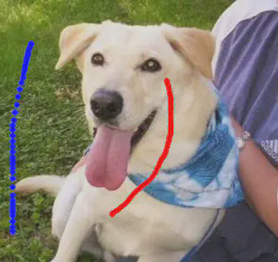
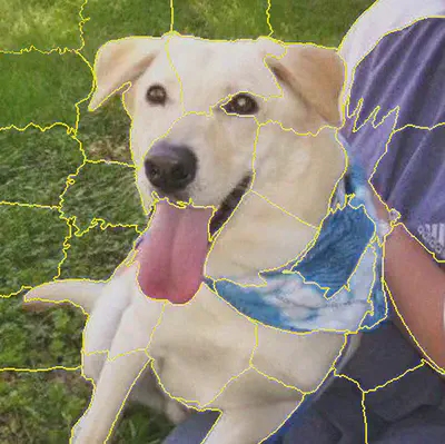
For the moment, ignore the blue and red curves. The point here is that we have no previous labeled data on how to perform such a classification, so we rely only on our prior knowledge. To make things simpler, we first perform a simple preprocessing step of extracting superpixels of the image. This procedure clusters nearby pixels with similar colors, for forming a partition of the image into larger regions. The result is shown in the image below.

As a simplifying assumption, assume that all pixels in a superpixel belong to the same class (foreground or background). We can thus associate to each superpixel a variable $X_i$ denoting its class (say, 1 for foreground, 0 for background). A common model of image segmentation is to consider that:

• similar adjacent regions (superpixels) are more likely to belong to the same class;
• dissimilar adjacent regions are less likely to belong to the same class;
• regions only exert influence in other non-adjacent regions by means of their neighbors (or neighbors of neighbors and so on).

The result is the undirected graph overlaid in the image below, where the nodes are placed at the regions centroid, and connected through blue edges. Notice the existence of edges only among adjacent regions. The intuition is that once the class of neighboring regions is revealed, the influence of the remaining regions on that region disappears.

We obtain a full specification of the model by associating edge potential function $\phi_{ij}(X_i,X_j)$ to each pair of adjacent regions $i$ and $j$. That function encodes the principles that similar regions tend to be of the same class, and dissimilar regions tend to be of different class: $$ \phi_{ij}(X_i=1,X_j=1)=\phi_{ij}(X_i=0,X_j=0)=\rho $$ for some parameter $\rho \geq 0$, and $$ \phi_{ij}(X_i=1,X_j=0)=\phi_{ij}(X_i=0,X_j=1)=\gamma $$ for $\gamma \geq 0$. These parameters can be estimated, for example, by comparing summaries of the characteristics of the pixels of each region (e.g., mean color, size, etc). For example, we can define $\rho = \exp( - |\bar{c}_i - \bar{c}_j| ) = 1-\gamma$, where $\bar{c}_k$ denotes the mean color in region $k$. More sophisticated schemes can induce a local model of (dis)similarity for the pixels of the two regions.

The joint probability distribution over all variables is then defined as $$ P(X_1=x_1,\dotsc,X_n=x_n) = \frac{1}{Z} \prod_{ij} \phi_{ij}(X_i=x_i,X_j=x_j) , $$ where $$ Z = \sum_{x_1,\dotsc,x_n} \prod_{ij} \phi_{ij}(X_i,X_j) $$ is a normalizing constant, whose purpose is to ensure that $P$ adds to one. We can now proceed in different ways to obtain a segmentation. A simple one is to find a configuration of the variables that maximize the joint distribution. We can also use the red/blue curves annotated in Figure 4 as evidence, to improve the quality of the solution (so that we are actually finding the most probable configuration consistent with the evidence). This result is shown in the image below.

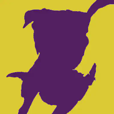
Another possibility is to compute the marginal probability $P(X_i=1|\text{evidence})$ for each pixel, and decide its class accordingly (foreground if and only greater than a given threshold, for example).

What else

In the rest of the course, we will formalize the directed and undirected graphical representation of independences, and discuss it leads to a computationally efficient procedure for deriving implied assumptions. We will study techniques for learning both the parameters and the graphical structure of a probabilistic model from data; we will study how to efficiently and accurately draw different inferences with a model. At last, we will investigate how these models can be extended to capture notions of causality. We start by reviewing the basics of probability theory.