Markov Networks
$ \newcommand{\nb}[1]{\text{ne}(#1)} \newcommand{\pa}[1]{\text{pa}(#1)} \newcommand{\ch}[1]{\text{ch}(#1)} \newcommand{\de}[1]{\text{de}(#1)} \newcommand{\an}[1]{\text{an}(#1)} \newcommand{\nd}[1]{\text{nd}(#1)} \newcommand{\can}[1]{\overline{\text{an}}(#1)} \newcommand{\ind}{⫫} \newcommand{\dsep}{\perp_d} \newcommand{\sep}{\perp_u} \newcommand{\msep}{\perp_m} $
We examine the representation of independence by undirected graphs, resulting in the concept of Markov networks. We also compare Bayesian networks and Markov networks as representational devices for independences.
A few more concepts from graph theory
Recall that an undirected graph is a pair $G=(V,E)$ where $E$ is a set of unordered pairs of vertices. We denote an undirected edge as $X-Y \in E$. A loop (or undirected cycle) is a trail that starts and ends with the same node. An undirected graph with no loops is a tree (even if it is not connected), otherwise it is loopy. A triangle is a 3-node loop. Here is an important class of graphs:
A graph is chordal if every loop has a subsequence which is a triangle.
The figure below shows a chordal graph on the left (any permutation of the loop $A,B,C,D$ has loops $A,B,C$ or $B,C,D$) and non-chordal graphs in the center and right (e.g., in the graph in the center the loop $A,B,C,D$ has no subsequence which is also a loop). Note that the rightmost graph is non-chordal even though is made up of triangles. The outer loop $A,B,C,D,E,F$ contains no triangles.

The following concept will be central for our discussion.
A clique is a set of nodes which are pairwise connected. A clique is maximal if it is not a proper subset of any other clique.
The maximal cliques of the left graph in the figure above are $\{A,B,C\}$ and $\{B,C,D\}$ and the non maximal cliques are the edges, the singletons containing each node and the empty set. The maximal cliques of the graph in the center are its edges. The maximal cliques of the graph on the right are the triangles, all containing node $G$.
Markov networks
We have seen that even though independence is a symmetric concept, it can be well captured by an acyclic directed graph through the semantics of d-separation. Moreover, we saw that d-separation is equivalent to m-separation, thus connecting directed and undirected representations. The m-separation representation, obtained through the relevant moral graph, is dynamic in that it depends on a graph constructed specifically for the desired independence (or separation) query. In this section we will look at a undirected representation of independence that is static, that is, it is represented by a fixed graph.
Motivation
Let us motivate the undirected graphical representation of independences by a simple example.
Contact networks (a.k.a mixing networks or diffusion networks) are commonly used to represent the spread of infectious diseases in heterogeneous populations. They are also used to represent more general diffusion processes, such as the transmission of information (e.g. hoaxes), or natural processes such as wildfires. A contact network is an undirected graph whose nodes represent individuals and edge represent potential interaction among individuals. For instance the graph below represents contact patterns among four individuals.

Associate to each node $X$ a binary random variable indicating whether a person is infected or not. We are interested in building a model for all individuals; in the simple case of the graph above, that amounts to specifying $P(A,B,C,D)$. Assuming that infection occurs only though interactions between contacts, we have that $$ A \ind D \mid B,C, \quad B \ind C \mid A,D \, $$ and no other independence (at the variable level). That means, for example, that the probability that $A$ is infected given that $D$ is infected is obtained by $$ P( A = 1 \mid D =1) = \sum_{B,C} P(A=1 \mid B, C)P(B,C \mid D) \, . $$
Note that the independences in the model above cannot be represented using d-separation, as the presence of a immorality would make two non-adjacent variables independent by conditioning on a single adjacent node.
Separation
Independences in undirected graphs are read as standard separation (i.e., non-connectivity) in graphs:
The sets of variables $\mathcal{X}$ and $\mathcal{Y}$ are u-separated by $\mathcal{Z}$, written $\mathcal{X} \sep \mathcal{Y} \mid \mathcal{Z}$ if $\mathcal{X}$ and $\mathcal{Y}$ are separated in $G-\mathcal{Z}$.
Hence, m-separation is simply u-separation in the corresponding relevant moral graph. Note that conditioning can only separate sets, but never connect them (this is the static character of u-separation), in stark contrast to d-separation.
Consider the graph in the center in Figure 2; it encodes the u-separations $$ A \sep D \mid B,C \text{ and } B \sep C \mid A,D \, . $$
Definition
A Markov network is a pair $(G,P)$, where $G$ is an undirected graph over variables $\mathcal{V}$ and $P(\mathcal{V})$ is a joint distribution for $\mathcal{V}$ such that $$ \begin{align*} & \mathcal{X} \sep \mathcal{Y} \mid \mathcal{Z} \text{ only if } \mathcal{X} \ind \mathcal{Y} \mid \mathcal{Z} \, , & & \text{[global Markov property]} \end{align*} $$ for any subsets $\mathcal{X},\mathcal{Y},\mathcal{Z} \subseteq \mathcal{V}$.
Markov networks are also called Markov Random Fields, following their usage in Physics.
The maximal cliques of the graph in Figure 2 are formed by the edges. Assuming the distribution is positive, the Markov network in the previous example factorizes as $$ P(A,B,C,D) \propto \phi(A,B)\phi(A,C)\phi(B,D)\phi(C,D) \, . $$ The clique potentials model the higher probability attributed to neighboring individuals having the same status (infected or not infected), plus any additional information about the status of an individual (e.g., the result of an imperfect test or a random chance of being infected by an exogenous phenomenon).
The Hammersley-Clifford Theorem
Our goal is to connect independences and factorizations, as we have done for directed graphs. This leads to the concept of a potential.
A potential is a nonnegative real-valued function over the joint domain of some set of variables.
A potential is also often called a factor and less often a valuation. Note that a (conditional) joint mass function or density is a potential (and the converse is not generally true). We say that a joint distribution $P(\mathcal{V})$ is positive if its corresponding joint mass function or density is positive (and more generally, for mixed-discrete continuous models, if the product of conditional density and mass function is positive). The parametrization of a Markov network in terms of potentials follows from the following result.
Hammersley-Clifford Theorem.
Let $\mathcal{C}_1,\dotsc,\mathcal{C}_m$ be the maximal cliques of a Markov network structure. If the joint distribution $P(\mathcal{V})$ is positive then the global Markov property implies that
$$ P(\mathcal{V}) = \frac{1}{Z}\prod_{j=1}^m \phi_j(\mathcal{C}_j) \, , $$
where
$$ Z = \sum_\mathcal{V} \prod_{j=1}^m \phi_j(\mathcal{C}_j) $$
is a normalizing term called the partition function.
The potentials $\phi_j$ are called clique potentials.
Factorization
It is possible to construct a non-positive distribution that satisfies all the global Markov properties in the graph and yet does not factorize over the cliques. The converse result (i.e., soundness), however, holds even for non-positive distributions.
If $P(\mathcal{V})$ is a joint distribution that factorizes as $$ P(\mathcal{V}) = \frac{1}{Z}\prod_{j=1}^m \phi_j(\mathcal{C}_j) \, , $$ where $\mathcal{C}_j$ are the maximal cliques of a graph $G$, then $(G,P)$ satisfies all the global Markov properties.
The result above uses the following fact about independence:
The sets of variables $\mathcal{X}$ and $\mathcal{Y}$ are conditionally independent given the set of variables $\mathcal{Z}$ if and only if there are potentials $\phi_1(\mathcal{X},\mathcal{Z})$ and $\phi_2(\mathcal{Y},\mathcal{Z})$ such that $$ P(\mathcal{X},\mathcal{Y}) = \phi_1(\mathcal{X},\mathcal{Z}) \phi_2(\mathcal{Y},\mathcal{Z}) \, . $$
Markov properties
It is not difficult to show that Global Markov properties imply
Local Markov property:
$$ X \sep \mathcal{V} - \nb{X} \mid \nb{X} \text{ only if } X \ind \mathcal{V} - \nb{X} \mid \nb{X} \, . $$
The property above implies that
Pairwise Markov property:
$$ X-Y \not\in E \text{ only if } X \ind Y \mid \mathcal{V} - \{X,Y\} \, . $$
For positive Markov Networks, the converse implications are also valid:
If $P(\mathcal{V})>0$ the following tree assertions are equivalent.
- $P$ satisfies the pairwise Markov property:
$$ X \sep Y \mid Z \implies X \ind Y \mid Z \, . $$
- $P$ satisfies the local Markov property.
$$ X \sep V-\nb{X} \mid \nb{X} \implies X \ind V-\nb{X} \mid \nb{X} \, . $$
- $P$ satisfies the global Markov property.
Note that unlike Bayesian networks, we defined Markov networks satisfying the global Markov properties from which we deduced the local Markov properties and the pairwise Markov properties. According to the result above, for positive distributions this choice is arbitrary: we could have defined Markov networks as satisfying the local or pairwise Markov properties, as we did with Bayesian networks. However, there are non-negative distributions which satisfy the pairwise Markov properties and not the local Markov properties, and distributions which satisfy the local Markov properties and not the global ones.
When the distribution is positive, it is also common to parametrize it using a distribution from the exponential family: $$ P(\mathcal{V}) = \frac{1}{Z} \exp \left ( -\sum_j \psi_j(\mathcal{C}_j) \right ) = \exp\left ( -\sum_j \psi_j(\mathcal{C}_j) - \ln(Z) \right ) \, , $$ where $\psi_j = \ln 1/\phi_j $ are clique log-potentials. A distribution satisfying the equation above is often called a Gibbs distribution. The term $$ \sum_j \psi_j(\mathcal{C}_j) $$ is often called energy function of the model.
Here is an example of use of a Gibbs distribution over continuous variables.
This example was taken from Kevin Murphy’s book (page 115),1 which in turn was based on example by Calvetti and Somersal 2007’ book.2 Consider the task of interpolating a given (noise-free) data set. To make it more concrete, assume the data represented by the larger circles in the plot below.

We assume that the data was generated from a sufficiently smooth function $y=f(x)$ (i.e., differentiable, with small first and second derivatives). We divide each interval of consecutive data points $[x_i,x_{i+1})$, $i=1,\dotsc,8$, into uniformly spaced points $x_j$ such that $$ x_{j+1} \approx x_j + h \, $$ where $h > 0$ is some parameter of our model that describes the quality of the discretization. The values $x_j$ when $h=0.1$ are shown as the smaller black circles laid out at $y=0$ in the plot above. For each such point, we let $y_j = f(x_j)$ denote the corresponding mapping through the unknown function $f$. To simplify the notation, assume a relabeling of the indices so that the combination of the observed data points and the newly created points are denoted as $$ X_1,X_2,\dotsc,X_n \, . $$ The task is to construct a joint distribution of the continuous variables $Y_1,\dotsc,Y_n$. The smoothness of the function can be encoded in discrete form as $$ (y_{i+1} - y_{i})/h \approx (y_i - y_{i-1})/h \, . $$ Canceling out the common $1/h$ factor, and rearranging terms, we obtain $$ 2y_i \approx y_{i-1} + y_{i+1} \, . $$ We can model the knowledge above by three-place log-potentials $$ \psi_j(y_{j-1},y_j,y_{j+1}) = \gamma \left ( 2y_j - y_{j+1} - y_{j-1} \right )^2 \, , $$ where $\gamma > 0$ is a parameter describing the smoothness of the interpolation. The potential above enforces configurations where $y_j$ is close to the mean of $y_{j-1}$ and $y_{j+1}$. The joint Gibbs distribution is given by $$ P(Y_1,\dotsc,Y_n) = \exp\left( -\gamma \sum_{j=2}^{n-1} ( 2y_j - y_{j+1} - y_{j-1})^2 ) - \ln Z \right) \, . $$ We can use the model to obtain probable interpolations consistent with the given datapoints, and calculate their corresponding probabilities. The figure belows whose the original curve in red used to sample the datapoints and a probable interpolation, in black, consistent with the observed data, generated by Gibbs sampling.

Pairwise Markov networks
The Hammerley-Clifford Theorem requires potentials to be defined over maximal cliques. In many applications however it is parametrize such potentials in terms of smaller potentials. Here is a common class of Markov networks with a linear number of parameters in the number of edges:
A pairwise Markov network is a Markov network whose maximal cliques are the edges of the graph. It is commonly parametrized as $$ P(\mathcal{V}) = \exp\left( -\sum_{X \in \mathcal{V}} \psi(X) -\sum_{X-Y} \psi(X,Y) - \ln(Z) \right ) \, , $$ where $\psi(X)$ and $\psi(X,Y)$ are called the node and edge potentials, respectively.
The formulation in terms of log-potentials $\psi$ is not relevant (and is often avoided to represent logical constraints). Pairwise Markov networks are widely used in representing spatial information such as images and linked data.
Image segmentation is the task of grouping pixels of an image according to a pre-determined set of labels (e.g., foreground, background). Every pixel is classified according to local characteristics (pixel intensity, color, position, etc), and a spatial smoothing is enforced (neighboring pixels have similar classes). This model is often represented as a pairwise Markov where every pixel is a node and two nodes are adjacent if they correspond to adjacent pixels. The graph below represents a pairwise Markov network model of a 3-by-4 pixel image.
As a more concrete example, consider segmenting the image below into foreground and background classes.
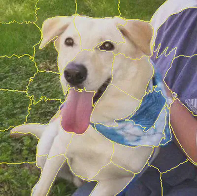
The yellow lines are generated by a preprocessing step that clusters nearby pixels with similar color. The corresponding regions are known as superpixels. This process can be seen as a dimensionality reduction of the data, and is used to simplify computations. We assume that all pixels of a superpixel have the same label, and associate each region to a variable $X_i$ taking values 0 and 1. Let $\bar{x}_i$ denote an aggregate statistic of the pixels in region $X_i$, for example, its mean intensity. The spatial smoothness is enforced through edge potentials $\psi$ defined as
$$ \psi(X_i=1,X_j=1) = \psi(X_i=0,X_j=0) = \rho|\bar{x}_i - \bar{x}_j| $$
for some parameter $\rho \geq 0$, and
$$ \psi(X_i=1,X_j=0) = \psi(X_i=0,X_j=1) = \gamma|\bar{x}_i - \bar{x}_j| $$
for some $\gamma \leq 0$. Note that $|\bar{x}_i - \bar{x}_j|$ is a constant in the expressions above.
The joint probability distribution over all variables is then defined as
$$ P(X_1=x_1,\dotsc,X_n=x_n) = \exp\left( - \sum_{X_i-X_j} \psi(X_i,X_j) - ln Z\right)\, , $$
where
$$ Z = \sum_{x_1,\dotsc,x_n} \exp\left( - \sum_{X_i-X_j} \psi(X_i,X_j) \right ) \, . $$
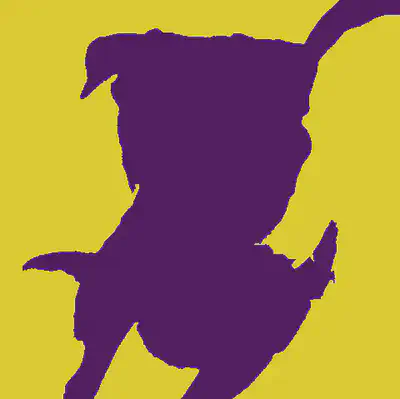
The figure below shows the result of the most probable segmentation.
Reduced Markov networks
A restriction of a potential $\phi(\mathcal{X},\mathcal{Y})$ with respect to an assignment $\mathcal{Y}=y$ is the potential $\phi_{\mathcal{Y}=y}(\mathcal{X})$ such that $\phi(x,y) = \phi_{\mathcal{Y}=y}(x)$ for every configuration $x$.
When convenient we write $\phi(\mathcal{X},\mathcal{Y}=y)$ to denote the restriction $\phi_{\mathcal{Y}=y}(\mathcal{X})$.
The restriction of the potential
| $X$ | $Y$ | $\phi(X,Y)$ |
|---|---|---|
| 0 | 0 | 0.1 |
| 0 | 1 | 100 |
| 1 | 0 | 5.2 |
| 1 | 1 | 0 |
with respect to $Y=1$ is
| $X$ | $\phi(X,Y=1)$ |
|---|---|
| 0 | 100 |
| 1 | 0 |
Markov networks are closed with respect to restrictions:
If $(G,P)$ is a Markov network over $\mathcal{V}$ such that $P$ factorizes as
$$ \frac{1}{Z}\prod_j \phi_j(\mathcal{C}_j) \, , $$ $\mathcal{Y} \subseteq \mathcal{V}$ is a subset of the variables, and $y$ is a configuration for $\mathcal{Y}$ then $(G-\mathcal{Y},q)$ is a Markov network over $\mathcal{V}-\mathcal{Y}$ and $Q$ factorizes as
$$ \frac{1}{Z(y)} \prod_j \phi_j(\mathcal{C}_j-\mathcal{Y}, \mathcal{Y}=y) \, . $$
Moreover, $$ Q(\mathcal{X})=P(\mathcal{X}|\mathcal{Y}=y) $$ for any $\mathcal{X} \subseteq \mathcal{V} - \mathcal{Y}$.
The Markov network $Q$ is called a reduced Markov network. The notation $Z(y)$ emphasizes that the partition function of the reduced network depends on the restriction. Hence, computing conditional probabilities in Markov networks is the same as restricting every potential with respect to the observation and then computing a marginal probability (which requires computing the partition function). Note that the maximal cliques in the reduced network may be smaller than in the original network, so that more than a potential must be combined to form the clique potentials of the reduced network.
Consider a Markov network with the graph in the left in Figure 1, and its restriction by $B=1,C=0$. The corresponding reduced network is an empty graph over nodes $A$ and $D$, and the clique potentials are $$ \phi_1(A)=\phi(A,B=1)\phi(A,C=0) $$ and $$ \phi_2(D)=\phi(B=1,D)\phi(C=0,D) \, . $$ Note that the potential $\phi(B,C)$ is discarded (since it is a constant in the reduced model). Alternatively, $\phi(B=1,C=0)$ could be incorporated into any clique potential (or all of them). The reduced network distribution is $P(A,D|B=1,C=0)$.
Chordal graphs
Since any Bayesian network factorizes (even the ones with zero probability values), a Bayesian network $(G,P)$ specifies a Markov network $(M(G),P)$ whose partition function is $Z=1$ (however the set of independences encoded by both representations differ). Hence, from the parametrization point-of-view, Bayesian networks are subclass of Markov networks with the special property that the partition function is one. However, Bayesian networks can represent dynamic independencies (i.e., independencies created by conditioning), whereas Markov networks can represent only static dependencies. So, for example, no Markov network can represent the independencies in a convergent connection. Conversely, there are independence relations that can be represented by a Markov network but not by any Bayesian network. This is the case, e.g., of the network in the center in Figure 1. Any attempt of representing that relation as a directed graph will either result in creating a convergent connection which misses some independence and introduces others, or lack a direct influence (again, misrepresenting independences). Thus, from the representational point-of-view, Bayesian networks and Markov networks are incomparable.
What types of independence relations can be represented either by a directed or an undirected graph? The answer follows from our translation from Bayesian networks to Markov networks. Recall that the equivalence class of a Bayesian network is characterized by the skeleton and the set of immoralities. A Bayesian network without immoralities is thus represented as an undirected graph, in which case d-separation (with any consistent orientation of the arcs) and u-separation coincide. So the class of Bayesian networks such that $G=M(G)$ is contained in the class of Markov networks. What about the converse? Any triangle-free loop contains independences that cannot be represented by a directed graph (consider the graph in the center in Figure 1). On the other hand, any triangle

can be represented either as the directed structure

or by any isomorphic structure. Combining these arguments, one can show that the class of Markov networks that can be represented as Bayesian networks is exactly the class of chordal graphs; any non-chordal graph cannot be represented (in terms of independences) by a Bayesian network.
Let $G$ be an undirected graph. The following statements are equivalent:
- G is chordal.
- There is an acyclic directed graph $D$ such that $M(D)=G$.
- There is an acyclic directed graph $D$ such that $\mathcal{X} \dsep \mathcal{Y} \mid \mathcal{Z}$ if and only if $\mathcal{X} \sep \mathcal{Y} \mid \mathcal{Z}$.
The equivalences between Bayesian and Markov networks are represented in the figure below. As is noted in the diagram, trees are particular cases of chordal graphs.

Clique Tree Reparametrization
We will see later that chordal graphs, the intersection of Markov networks and Bayesian networks are an important family of probabilistic graphical models, one in which inference complexity can be graphically characterized. Chordal graphs have the important property that their cliques can be arranged in the form of a tree with certain properties, and parametrized as $$ P(\mathcal{V}) = \frac{\prod_{j=1}^m P(\mathcal{C}j)}{\prod{j=1}^{m-1} P(\mathcal{S}_j)} \, , $$ where $\mathcal{C}_j$ are the cliques of the graph and $\mathcal{S}_j$ are the intersection of adjacent cliques known as separation sets.
Representation power
Since the restriction of potentials of a Markov network is also a Markov network, and a Bayesian network parametrizes a Markov network, we can compute conditional probabilities in Bayesian networks by inference in the corresponding restricted Markov network. Let $\mathcal{Y}=y$ be an evidence (i.e., an observation), and $\mathcal{X}$ be some target variables. To compute $P(\mathcal{X}|\mathcal{Y}=y)$ in a Bayesian network with graph $G$, obtain the potentials
$$ \phi_i = P_{\mathcal{Y}=y}(X_i|\pa{X_i}) $$
and compute the marginal $Q(\mathcal{X})$ in the Markov network defined by the factorization
$$ Q(\mathcal{V}-\mathcal{Y})=\frac{1}{Z}\prod_i \phi_i \, . $$
The partition function of this network encodes $Z=p(\mathcal{Y}=y)$, that is, the probability of the evidence. To make things computationally more efficient, we can restrict the Markov network to non-barren nodes with respect to $\mathcal{X}$ and $\mathcal{Y}$, which are exactly the ancestors of $\mathcal{X}$ and $\mathcal{Y}$ in $G$.