CoGA manual

1. Loading the dataset
2. Setting the parameters and running the analysis
3. Interpreting the results
4. Further Analyses
5. Running CoGA from the command-line interface
6. References

1. Loading the dataset

To run CoGA, you must upload on the left sidebar files containing gene expression data, phenotype labels, and a collection of gene sets. Detailed information about the data formats are described below.

Gene expression data (*.txt)

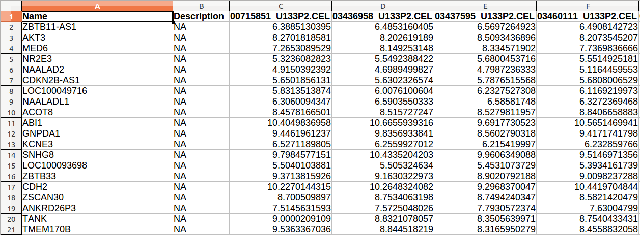
The expression data is a tab delimited file that contains the gene expression levels of all the samples. The first line has the following format:

  Name[tab][sample 1 name][tab][sample 2 name][tab] ...

It is allowed to include a Description field, which will be ignored. In that case, the first line is:

  Name[tab]Description[sample 1 name][tab][sample 2 name][tab] ...

Each line contains the gene (or probe set) name, the gene description (optional), and a value for each sample.

You can create the gene expression input file with a spreadsheet software, and then save it as a tab delimited text file. The final file must have the *.txt extension.

The figure below illustrates an expression input file:

Annotation data (*.chip)

If your dataset is already collapsed to gene symbols (i.e., the row identifiers are the gene symbols, and each gene is represented by a single row), just select the "Keep the original expression data rows" option and skip to the next section. Otherwise, select the "Collapse dataset to gene symbols" option, and then choose a method to summarize the rows (probe sets) representing the same gene by a single representative. The methods for collapsing are the same used in the WGCNA package (Langfelder and Horvath, 2008), which we describe below:

• MaxMean: choose the row with the highest mean value
• MinMean: choose the row with the lowest mean value
• AbsMaxMean: choose the row with the highest mean absolute value
• AbsMinMean: choose the row with the lowest mean absolute value
• MaxRowVariance: choose the row with the highest variance
• ME: choose the eigenrow (first principal component of the rows that represent the same gene)
• Average: for each column, take the average value of the rows that represent the same gene

If the "Connectivity based collapsing" option is "True", the collapsing procedure is:

If a gene has exactly two corresponding probe sets, then it chooses the row according to the selected collapsing method. If a gene has three or more corresponding probe sets, it computes the pairwise correlations among the rows that represent the same gene and then selects the highly correlated one.

For a detailed discussion about the collapsing methods described above, we refer to the Miller et al. (2011) paper.

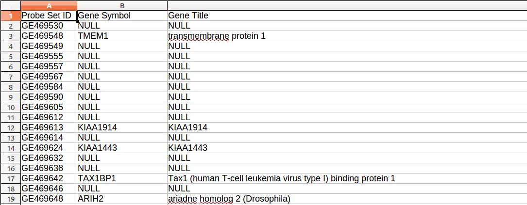
After selecting a collapsing method, upload an annotation file that maps the microarray probe set IDs to gene symbols. We recommend to use the GSEA microarray annotation files, which are freely available at the Broad ftp site (ftp://gseaftp.broadinstitute.org/pub/gsea/annotations).

The annotation file has three columns separated by tabulations. The first line has the following format:

 Probe set ID[tab]Gene symbol[tab]Gene title

The figure below illustrates an annotation file:

Phenotype labels (*.cls)

The categorical class file identifies the phenotype class that each sample belongs to. It is a text file delimited by blank spaces. The file must contain tree lines and the *.cls extension.

The first line has the number of samples and classes (phenotypes), and the number one, in that order. The second line has the "#" symbol followed by the class names. The third and last line contains a class label for each sample. You can use any symbol for the labels (a number, text, or the same name you have specified on the previous line). The first label corresponds to the first class that appears on the second line; the second label corresponds to the second class; and so on.

Below, we show the cls file format:

  [number of samples][space][number of classes][space]1
  # [space][class 1 name][space][class 2 name]
  [sample 1 class][space][sample 2 class][space] ... [sample N class]

Consider that you want to analyze 65 samples from the class AII and 30 samples from the class ODII. If the first columns of the gene expression matrix correspond to the AII microarrays and the last ones to the ODII microarrays, then the cls input could be:

  95 2 1
  # AII ODII
  0 0 0 0 0 0 0 0 0 0 0 0 0 0 0 0 0 0 0 0 0 0 0 0 0 0 0 0 0 0 0 0 0 0 0 0 0 0 0 0 0 0 0 0 0 0 0 0 0 0 0 0 0 0 0 0 0 0 0 0 0 0 0 0 0 1 1 1 1 1 1 1 1 1 1 1 1 1 1 1 1 1 1 1 1 1 1 1 1 1 1 1 1 1 1

Here, "0" indicates de samples belonging to class AII, and "1" indicates the samples belonging to ODII.

Gene set database (*.gmt)

The gene set database file describes the groups of genes that will be analyzed. The columns are tab delimited. Each row corresponds to a gene set. The first column describes the gene set name, the second one contains a gene set description, and the following columns contain the genes that belong to the set. The file must have the *.gmt extension and is illustrated by the figure below:

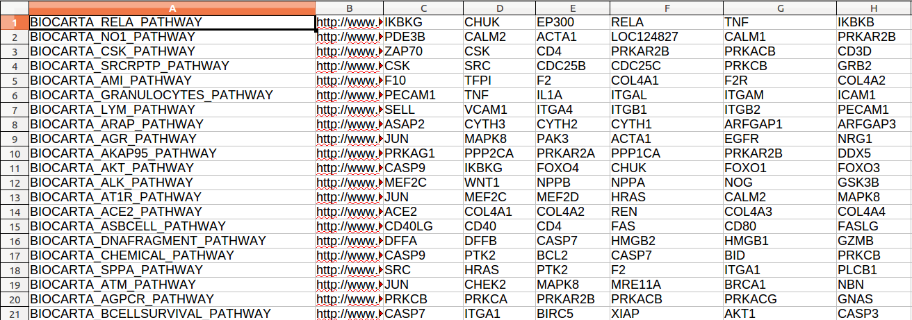
Several gmt format gene set collections are freely available at the Molecular Signature Database (MSigDB) (http://www.broadinstitute.org/gsea/msigdb/index.jsp) (Subramanian et al., 2005).

2. Setting the parameters and running the analysis

Before running CoGA, you must set the execution parameters available on the left sidebar. Below, we detail each differential network analysis parameter.

Classes (conditions) being compared

CoGA analyses compare only two phenotypes. If your dataset has more than two phenotypes, then you must select one pair of phenotypes from a list of all possible pairs.

The selected pair will be used by all CoGA analyses.

Gene sets size range

CoGA performs tests for each gene set of a collection of gene sets. To test only a subcollection of sets, you can filter the gene groups according to their sizes by setting the "Minimum gene set size" and "Maximum gene set size" parameters.

The minimum gene set size allowed is 2. However, we recommend to test groups with at least 20 genes.

Testing large gene sets can spend much time. In general, it is feasible to set 1000 or some hundreds of genes as the maximum gene set size. However this number may vary according to the user's machine specification.

Method for network inference

The network links are inferred according to a measure of association between the gene expression levels. CoGA provides three classical association measures:

• Pearson: Pearson's correlation coefficient. It measures the linear dependence between two variables. For the statistical test, we use the Hmisc package.
• Spearman: Spearman's correlation coefficient. It measures the monotonic dependence between two variables. For the statistical test, we use the Hmisc package.
• Kendall: Kendall's Tau coefficient. It measures the monotonic dependence between two variables. For the statistical test, we use the psych package.

The correlation coefficient or p-value obtained by one of the methods mentioned above are used to set an association degree for each link of the network. The following options are available to measure the association degrees:

• Absolute correlation: the absolute value of the correlation coefficient
• 1 - p-value: One minus the p-value of the test for dependence between two gene products. If the p-value is small, the expression levels are tightly associated.
• 1 - q-value: One minus the adjusted p-value of the test for dependence between two gene products. The p-value is adjusted by the False Discovery Rate (Benjamini and Hochberg, 1995) method for multiple testing.

Network type

You can choose between unweighted and weighted networks:

• Unweighted: Graphs where all the edges are weighted by one. You must choose a threshold for the edges selection. Only the edges that connect genes with an association degree greater than the threshold will remain in the graph.
• Weighted: Weighted networks are full graphs where each edge has a weight. The weight of an edge is defined as the association degree between the two gene products that are connected by it.

Method for gene networks comparison

CoGA compares the gene co-expression networks between two phenotypes for each gene set.

Below, we describe the methods available for comparing unweighted networks:

• Spectral distribution test: The spectrum of an undirected graph is the set of eigenvalues of its adjacency matrix. The spectrum distribution describes many topological properties of a graph, such as the number of walks, diameter, and cliques. The spectral distribution test is based on the Jensen-Shannon divergence between spectral distributions (Takahashi et al., 2012). It can be used to test if two graphs were generated by the same model.
• Spectral entropy test: It uses the absolute difference between spectral entropies (Takahashi et al., 2012) to measure the difference in the graph topological organization complexity.
• Degree distribution test: The degree of a node is the number of edges that connect to it. The degree distribution test is based on the Jensen-Shannon divergence between the degree distributions. CoGA uses the igraph package implementation of the node degree.
• Degree centrality test: The degree centrality test is based on the Euclidian distance between the degree centralities of the two networks adjusted by the number of vertices.
• Betweenness centrality test: The betweenness centrality of a node is the number of shortest paths going through it (Freeman, 1979). The betweenness centrality test is based on the Euclidian distance between the betweenness centralities of the two networks adjusted by the number of vertices. CoGA uses the igraph package implementation.
• Closeness centrality test: The closeness centrality of a node is the inverse of the average length of the shortest paths between it and all the other vertices in the graph (Freeman, 1979). The closeness centrality test is based on the Euclidian distance between the closeness centralities of the two networks adjusted by the number of vertices. CoGA uses the igraph package implementation.
• Eigenvector centrality test: The eigenvector centrality of a node v_i is the ith value of the first eigenvector of the graph adjacency matrix (Bonacich, 1987). The eigenvector centrality test is based on the Euclidian distance between eigenvector centralities of the two networks adjusted by the number of vertices. CoGA uses the igraph package implementation.
• Clustering coefficient test: The local clustering coefficient of a node is the number of edges between the vertices within its neighborhood divided by the number of edges that could exist among them (Watts and Strogatz, 1998). The clustering coefficient test is based on the Euclidian distance between the local clustering coefficients of the two networks adjusted by the number of vertices. CoGA uses the igraph package implementation.
• Shortest path length test: The shortest path length test is based on the absolute difference between the averages of all the shortest path lengths for all pair of nodes v_i and v_j with i ≠ j. CoGA uses the igraph package implementation.

CoGA includes generalizations of some of the statistics described above to weighted undirected graphs. Let G be a weighted undirected graph. We define the weighted adjacency matrix of G to be the matrix W = (w)_ij, such that w_ij is the weight of the edge that connects the vertices v_i and v_j. In this context, 0 ≤ w_ij ≤ 1 and G is a full graph.

Below, we describe the methods available for comparing weighted networks:

• Spectral distribution test: Replaces the usual adjacency matrix by the weighted adjacency matrix, and then performs the spectral distribution test for unweighted networks.
• Spectral entropy test: Replaces the usual adjacency matrix by the weighted adjacency matrix, and then performs the spectral entropy test for unweighted networks.
• Degree distribution test: CoGA generalizes the degree of a node to the sum of the weights of the edges that connect to it (Barrat, 2004). The software uses the igraph implementation of the node strength. It replaces the usual node degree by the weighted degree, and then computes the degree distribution test for unweighted networks.
• Degree centrality test: Replaces the usual node degree by the weighted degree, and then computes the degree centrality test for unweighted networks.
• Eigenvector centrality test: replaces the usual adjacency matrix by the weighted adjacency matrix, and then performs the eigenvector centrality test for unweighted networks (Newton, 2004).
• Clustering coefficient test: replaces the local clustering coefficient of a node by the sum of the weights of the edges between the vertices within its neighborhood divided by the number of edges that could exist among them (Lopez-Fernandez et al, 2004). Then it performs the clustering coefficient test for unweighted networks.

For the "Spectral distribution test", the "Spectral entropy test", and the "Degree distribution test" methods, you must select a criterion to define the bandwidth for the probability density function estimation. The available methods for computing the bandwidth are:

• Sturges: the bandwidth is defined as (max(x) - min(x))/n_bins (Sturges, 1926), where x is the graph spectrum (for the tests based on the spectral density) or the node degrees (for the degree distribution test), and n_bins=⌈log₂(n_V) + 1⌉, with n_V denoting the number of genes.
• Silverman: the bandwidth is defined as 0.9min{sd(x), IQR(x)/1.34} n_V^-0.2 (Silverman, 1986), unless the quartiles coincide, where n_V is the number of genes, sd(x) is the standard deviation of x, and IQR is the interquantile range of x, with x denoting the graph spectrum (for the tests based on the spectral density) or the node degrees (for the degree distribution test). If the graph is empty, it is defined as 0.9n_V^-0.2.

CoGA uses the R 'density' function from the base package for estimating the probability density function.

Permutation test settings

To compute a p-value for the differential network analysis, CoGA performs a permutation based test, which generates N random permutations of the sample labels.

The minimum possible p-value is ¹⁄_{N + 1}. Therefore, the choice of N depends on the required significance level of the test. You can set the N parameter on the "Enter the number of label permutations" option.

To perform the same label permutations for all gene sets, you can set a seed to generate the random permutations on the "Enter a seed to generate random permutations" option.

Running the analysis

After loading the dataset and the execution parameters, click on the "Start analysis" button. A progress bar will be shown on the right top corner of the page:

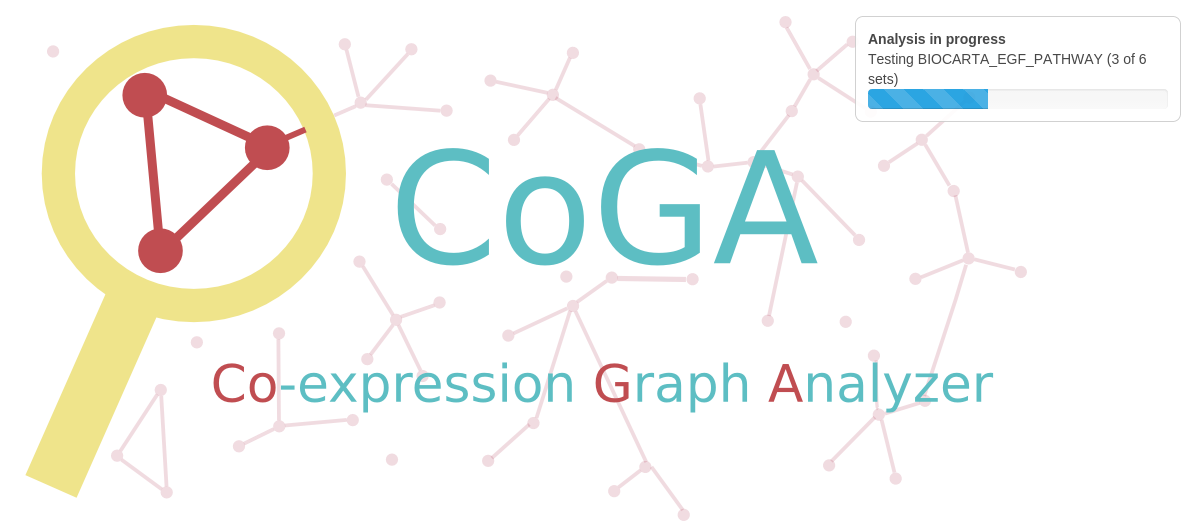
The results and other execution messages are shown on the "Analysis results" section.

3. Interpreting the results

When the differential network analysis finishes, the results are shown on the "Analysis results" tab.

Results table

The results table has the following format:

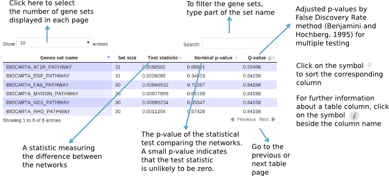
You can save the results as a CSV or R data file:

• CSV: a comma-separated text file, containing the execution parameters and the results table. It can be opened with a spreadsheet software
• R data: a file that contains two R variables: a data frame called "results" (the differential network analysis results), and a table called "parameters" (the parameters used in the analysis). It can be loaded using the "load" command in the R console.

Missing p-values

The differential network analyses may fail when empty graphs are inferred from the expression data. Missing p-values are likely to happen for unweighted small graphs.

If you are using the "Spectral entropy test", the "Spectral density test", or the "Degree distribution test", setting the bandwidth to Silverman's criteria will avoid the missing p-values.

If you are using the "Shortest path test", the analysis will always fail when the graph is empty. To avoid it, try filtering larger gene sets.

4. Further Analyses

After performing the differential network analysis, you can explore several gene set properties on the "Further analysis" tab.

Below, we explain the available tools for exploring the gene sets.

Gene set selection

To analyze a gene set, select it from the list of gene sets on the "Further analysis" tab. The following options are available for filtering the lists of gene sets:

• All gene sets with p-values less than the threshold: filter the gene sets with the network comparison test nominal p-value less than the selected threshold. This option is visible only after the differential network analysis finishes.
• All gene sets with q-values less than the threshold: filter the gene sets with the differential network test adjusted p-value by False Discovery Rate method (Benjamini and Hochberg, 1995) for multiple testing less than the selected threshold. This option is visible only after differential network analysis finishes
• All tested gene sets: the gene sets that were tested for the differential network analysis. This option is visible only after differential network analysis finishes.
• All filtered gene sets: the gene sets that were filtered according to their size on the left side panel. This option is visible only if differential network analysis has not been performed yet.
• All loaded gene sets: all gene sets of the uploaded gene set collection.

After selecting a gene set, choose a tab on the "Further analysis" section for analyzing the selected set.

Network visualization plots

Given a gene set name, the "Network visualization plots" tab on the "Further analysis" section provides tools to visually inspect the networks and the differences between the two phenotypes.

Below, we describe the available tools.

Plot settings

• Colors selection: select a color scheme for the plots
• Plot format: select a file format to save the plots
• Plot dimensions: set the plot dimensions in inches (for PDF format) or pixels (PNG and JPG formats)

Network visualization

The network visualization tool plots one association matrix for each phenotype.

The association matrix contains the association degree of each pair of genes from the selected gene set. The associations degrees are measured from the expression data using the method selected on the left sidebar ("Method for network inference"). The degrees vary between 0 and 1, and are represented by colors. If the "absolute correlation" option is selected on the sidebar, the user can visualize both absolute and non absolute correlations by setting the "Show negative correlations" option. To save the plots, click on the "Save class 1 network plot" and "Save class 2 network plot" buttons.

You can check out the value of each association degree on the "Association between two gene products" section.

Differences between the gene networks

To visualize the differences between the networks, you can plot a matrix of the differences. Each position of the matrix shows the difference in the correlation (association degree) of two gene products between the two phenotypes.

You can choose one of the following options:

• [class1] - [class2]: class1 association degree matrix minus class2 association degree matrix.
• [class2] - [class1]: class2 association degree matrix minus class1 association degree matrix.
• Absolute differences between the association degrees: matrix of the absolute values of the differences between the association degrees.

To plot the selected matrix of differences, just expand the "Matrix of differences" collapsing panel. You can save the plot by clicking on the "Save plot button".

To see the differences in association degree of each pair of genes, expand the "List of gene association degrees" collapsing panel. You can save the list as a CSV or R data file:

• CSV: a comma-separated text file, containing the association degrees between the gene products. It can be opened with a spreadsheet software
• R data: a file that contains a data frame R variable called associationDegrees. It can be loaded using the "load" command in the R console.

Gene set properties

To check out network features of each phenotype, select one of the options described below.

Network features for unweighted graphs:

• Spectral entropy: measures the graph topological organization complexity (Takahashi et al., 2012).
• Average degree centrality: The degree of a node is the number of edges that connect to it. The average degree centrality is the sum of all node degrees divided by the number of vertices.
• Average betweenness centrality: The betweenness centrality of a node is the number of shortest paths going through it (Freeman, 1979). The average betweenness centrality is the sum of all node betweenness centralities divided by the number of vertices.
• Average closeness centrality: The closeness centrality of a node is the inverse of the average length of the shortest paths between it and all the other vertices in the graph (Freeman, 1979). The average closeness centrality is the sum of all node closeness centralities divided by the number of vertices.
• Average eigenvector centrality: The eigenvector centrality of a node v_i is the ith value of the first eigenvector of the graph adjacency matrix (Bonacich, 1987). The average eigenvector centrality is the sum of all node eigenvector centralities divided by the number of vertices.
• Average clustering coefficient: The local clustering coefficient of a node is the number of edges between the vertices within its neighborhood divided by the number of edges that could exist among them (Watts and Strogatz, 1998). The average clustering coefficient is the sum of all node local clustering coefficients divided by the number of vertices.
• Average shortest path length: average of all the shortest path lengths for all pair of nodes v_i and v_j with i ≠ j.

Network features for weighted graphs:

• Spectral entropy: Replaces the usual adjacency matrix by the weighted adjacency matrix, and then computes the spectral entropy for unweighted networks.
• Average degree centrality: CoGA generalizes the degree of a node to the sum of the weights of the edges that connect to it (Barrat, 2004). It replaces the usual node degree by the weighted degree, and then computes the average degree centrality for weighted networks.
• Average eigenvector centrality: replaces the usual adjacency matrix by the weighted adjacency matrix, and then computes the average eigenvector centrality for unweighted networks (Newton, 2004).
• Average clustering coefficient: replaces the local clustering coefficient of a node by the sum of the weights of the edges between the vertices within its neighborhood divided by the number of edges that could exist among them (Lopez-Fernandez et al, 2004). Then it computes the average clustering coefficient for unweighted networks.

Gene scores

To rank the genes according to their ``importance'' in the networks, select one of the options below.

Gene scores for unweighted graphs:

• Degree centrality: The degree of a node is the number of edges that connect to it.
• Betweenness centrality: The betweenness centrality of a node is the number of shortest paths going through it (Freeman, 1979).
• Closeness centrality: The closeness centrality of a node is the inverse of the average length of the shortest paths between it and all the other vertices in the graph (Freeman, 1979).
• Eigenvector centrality: The eigenvector centrality of a node v_i is the ith value of the first eigenvector of the graph adjacency matrix (Bonacich, 1987).
• Local clustering coefficient: The local clustering coefficient of a node is the number of edges between the vertices within its neighborhood divided by the number of edges that could exist among them (Watts and Strogatz, 1998).

Gene scores for weighted graphs:

• Degree centrality: CoGA generalizes the degree of a node to the sum of the weights of the edges that connect to it (Barrat, 2004).
• Eigenvector centrality: replaces the usual adjacency matrix by the weighted adjacency matrix, and then computes the eigenvector centrality for unweighted networks (Newton, 2004).
• Local clustering coefficient: generalizes the local clustering coefficient of a node to the sum of the weights of the edges between the vertices within its neighborhood divided by the number of edges that could exist among them (Lopez-Fernandez et al, 2004).

You can save the gene scores as a CSV or R data file:

• CSV: a comma-separated text file, containing the gene scores. It can be opened with a spreadsheet software
• R data: a file that contains a data frame R variable called geneScores. It can be loaded by using the "load" command in the R console.

Gene expression analysis

Below, we describe the available single gene differential analysis tools.

Gene expression heatmap

The gene expression heatmap represents the gene expression levels by colors. Each column corresponds to a gene of the selected gene set, and each row represents one sample.

You can select the colors of the heatmap, and set its clustering options. The rows or columns of the heatmap will be clustered according to the enclidean distance. You can set the heatmap dimensions and save it as a PDF, PNG or JPG file.

CoGA uses the pheatmap CRAN package to plot the heatmaps.

Tests for differential expression

CoGA tests the difference in average or median expression levels of each single gene of the selected gene set. Those analyses use the "t.test" and "wilcox.test" R functions.

The figure below shows the table of results:

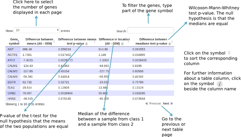
Those results can be saved as a CSV or R data file:

• CSV: a comma-separated text file, containing the differential analysis statistics and p-values. It can be opened with a spreadsheet software
• R data: a file that contains a data frame R variable called "diffExpressionAnalysis". It can be loaded by using the "load" command in the R console.

Gene expression boxplot

To visualize the distribution of the gene expression levels in each phenotype, just select a gene from the list on the "Gene expression boxplot" section.

You can set the plot dimensions and save it as a PDF, PNG or JPG file.

CoGA boxplots are built with the ggplot2 package.

5. Running CoGA from the command-line interface

CoGA analyses are also available in the R command line interface. Below, we describe how to perform the differential network analyses. For a detailed description of the function parameters and return values, check it out in the R command line interface, by typing the command ?[function_name].

Preparing the dataset

Read gene expression data

  expr <- readExprTxtFile([path_to_txt_file])

Read phenotype data

  labels <- readClsFile([path_to_cls_file], [class_1_name], [class_2_name])

Read annotation data

  annotation <- readChipFile([path_to_chip_file])

Collapse dataset to gene symbols

  collapsingMethod <- [collapsing_method_name]
  connectivityBasedCollapsing <- list("connectivityBasedCollapsing"=TRUE_or_FALSE)
  expr <- collapseExprData(expr, annotation, collapsingMethod, connectivityBasedCollapsing)

The available options for [collapsing_method_name] are:

• maxMean
• minMean
• absMaxMean
• absMinMean
• maxRowVariance
• me
• average

If [collapsing_method_name] is "me", the "connectivityBasedCollapsing" parameter will be ignored.

Read a collection of gene sets

  geneSets <- readGmtFile([path_to_gmt_file])

Setting the execution parameters

Network inference method

For using the absolute correlation coefficient as the association measure, create the following variables:

  networkInference <- [correlation_measure_name]Cor
  abs <- TRUE
  pvalue <- FALSE
  fdr <- FALSE

For using one minus the test p-value to measure the association between the gene products, create the following variables:

  networkInference <- [correlation_measure_name]Test
  abs <- TRUE
  pvalue <- TRUE
  fdr <- FALSE

For using one minus the test q-value as the association measure, create the following variables:

  networkInference <- [correlation_measure_name]Test
  abs <- TRUE
  pvalue <- TRUE
  fdr <- TRUE

The [correlation_measure_name] must be replaced by one of the following options:

• pearson
• spearman
• kendall

If your graph is weighted, you must set the following variables:

  weighted <- TRUE
  threshold <- NULL

If the graph is unweighted, then set them to:

  weighted <- FALSE
  threshold <- value

Replaces "value" by the desired threshold (only gene links with value higher then "value" will remain in the network).

Then, create the function for performing the network inference:

adjacencyMatrix <- adjacencyMatrix(networkInference, abs, pvalue, fdr, weighted, threshold)

Methods for comparing networks

  method <- [network_test_name]

If the graph is unweighted, the available values for [network_test_name] are:

• spectralDistributionTest
• spectralEntropyTest
• degreeDistributionTest
• degreeCentralityTest
• betweennessCentralityTest
• closenessCentralityTest
• eigenvectorCentralityTest
• clusteringCoefficientTest
• shortestPathTest

For weighted networks, the available methods are:

• spectralDistributionTest
• spectralEntropyTest
• degreeDistributionTest
• degreeCentralityTest
• betweennessCentralityTest
• closenessCentralityTest
• eigenvectorCentralityTest
• clusteringCoefficientTest
• shortestPathTest

Number of sample label permutations

  numPermutations <- [value]

Where [value] is the desired number of sample permutations

Seed for random permutations generation

To use different sample label permutations for each gene set, define the "seed" as NULL:

  seed <- NULL

Otherwise, set it to the desired value:

  seed <- [value]

Running differential network analysis

If [network_test_name] is "spectralDensityTest", "spectralEntropyTest" or "degreeDistributionTest" you must set a criterion for the bandwidth selection:

  options <- list("bandwidth"="Sturges")

or:

  options <- list("bandwidth"="Silverman")

To save the partial results in a file, set the parameter:

  resultsFile <- [path_to_results_file]

If [path_to_results_file] is NULL, then the partial results will not be saved.

To print execution messages, set the parameter "print" to TRUE:

  print <- TRUE

To perform the differential network analysis, type the command:

  results <- diffNetAnalysis(method, options, expr, labels, geneSets, adjacencyMatrix, numPermutations, print, resultsFile, seed)

6. References

Barrat, A. et al. (2004). The architecture of complex weighted networks. Proc. Natl. Acad. Sci. USA, 101, 3747.

Benjamini, Y. and Hochberg, Y. (1995). Controlling the false discovery rate: a practical and powerful approach to multiple testing. J. Roy. Statist. Soc. Ser. B, 57, 289-300.

Bonacich, P. (1987). Power and Centrality: A Family of Measures. Am. J. Sociol., 92, 1170-1182.

Freeman, L.C. (1979). Centrality in Social Networks I: Conceptual Clarification. Social Networks, 1, 215-239.

Langfelder, P. and Horvath, S. (2008). WGCNA: an R package for weighted correlation network analysis. BMC Bioinformatics, 9, 559.

Lopez-Fernandez, L. et al. (2004). Applying social network analysis to the information in CVS repositories. Proceedings of the 1st International Workshop on Mining Software Repositories (MSR '04), Edinburgh, Scotland, pp 101–105.

Miller, J. A. et al. (2011). Strategies for aggregating gene expression data: the collapseRows R function. BMC Bioinformatics, 12, 322.

Newman, M. E. J. (2001). Scientific collaboration networks. II. Shortest paths, weighted networks, and centrality. Phys. Rev. E, 64, 016132.

Newman, M. E. J. et al. (2004). Analysis of weighted networks. Phys. Rev. E, 70, 056131.

Silverman, B. W. (1986). Density Estimation. London: Chapman and Hall.

Sturges, H. A. (1926). The choice of a class interval. J. Amer. Statist. Assoc., 21, 65-66.

Subramanian, A. et al. (2005). Gene set enrichment analysis: A knowledge-based approach for interpreting genome-wide expression profiles. Proc. Natl. Acad. Sci. USA, 102, 15545-50.

Takahashi, D. Y. et al. (2012). Discriminating different classes of biological networks by analyzing the graphs spectra distribution. PLos One, 7, e49949.

Watts, D. J. and Strogatz S. (1998). Collective dynamics of 'small-world' networks. Nature, 393, 440–442.