PUMA's home page

How to Use

To run PUMA for estimating the thickness and the optical constants of a one-film system just type in a terminal the following sequence

puma FNAME NLAYERS SLAYER SUBSTRATE DATATYPE NOBS LAMBDAmin LAMBDAmax maxIT QUAD INIT THICKNESSmin THICKNESSmax THICKNESSstep INFLEmin INFLEmax INFLEstep N0ini N0fin N0step NFini NFfin NFstep K0ini K0fin K0step

where the capitalized words are parameters, described by

FNAME is a string (without blanks) representing the name of the film being studied. The input data file name must be in the format FNAME-dat.txt (the output file name will be automatically created adding "-inf.txt", so that is looks like FNAME-inf.txt). The input file should be structured as follows (see the example below):

a) the first line must contain the number of observations. If for example, you have 100 observations, the whole input file will have 101 lines.
b) from the second to the last line, it must contain, in each line, the wavelength and the transmittance (reflectance or both). This means that, from the second to the last line, there have to be either 2 or 3 numbers.
c) the observed data. i.e., transmittance (reflectance or both) has to be given in fractions, ranging from 0 up to 1. In this way, you must divide the measured data by 100 if they are given in percentages, ranging from 0 up to 100.
NLAYERS is the number of layers of the whole system, that is, the films, the substrate and the initial and final air layers. The present version works with only four layers, that is, one film. For systems with more than one film, see the parallel version of PUMA.
SLAYER is the number of the layer that corresponds to the substrate. For systems composed, from top to bottom, first air layer (layer 0), film (layer 1), substrate (layer 2) and last air layer (layer 3) set SLAYER equal to 2.
SUBSTRATE is a number describing the substrate. Use 10 for Corning 7059 glass substrate, 20 for crystalline silicon substrate, 30 for crystalline quartz substrate, 40 for glass slides substrate and 50 for borosilicate substrate.
DATATYPE is a character describing the data type. Use T for transmittance data, R for reflectance data and B for both.
NOBS is the number of points used in the optimization process. They are equally spaced points, interpolated inside the interval given by the parameters LAMBDAmin and LAMBDAmax (see below). This parameter is independent of the number of points furnished by the input file (FNAME-dat.txt).We strongly recommend you to use 100 points if you have not experience or are uncertain about this parameter.
LAMBDAmin is the left bound of the interval in which the optical constants will be estimated (LAMBDAmin must be greater than or equal to the smallest wavelength for which the measured data is provided in FNAME-dat.txt file).
LAMBDAmax is the right bound of the interval in which the optical constants will be estimated (LAMBDAmax must be smaller than or equal to the greatest wavelength for which the measured data is provided in FNAME-dat.txt file). Note that LAMBDAmax >= LAMBDAmin is mandatory.
MAXIT is the maximum number of iterations for the optimization solver. For each combination of fixed THICKNESS and INFLEPOINT (as determined in items 10 and 13) a nonlinear optimization problem is solved to estimate the optical constants and . We recommend you to use 3000 for the first trial, 5000 for the second trial, and 50000 for the last one.
QUAD is the quadratic error of the best optical constants estimation you have. Only quadratic error values smaller than QUAD are saved. In the first trial, we recommend to use a big number, such as 1e+100. When using the previous best estimation as the initial guess for a new trial, if may happen that, in this new trial, no better estimation is found. In this case, the returned retrieved thickness is zero.
INIT is an integer for choosing between either perform the initial estimative (in this case use 0), or use previous estimation as initial guess (in this case use 9). In the last case, i.e., when using the previously estimated optical constants to guide a new trial (INIT=9), the remaining parameters N0ini, N0fin, N0step, NFini, NFfin, NFstep, K0ini, K0fin and K0step are ignored.
THICKNESSmin is the trial thicknesses lower bound. This parameter, together with the next one must define an interval [THICKNESSmin,THICKNESSmax] inside of which you know that the real thickness you are trying to retrieve is. So, some kind of a priori knowledge of the thickness of the material is necessary to set this parameters.
THICKNESSmax is the trial thicknesses upper bound. Note that THICKNESSmax >= THICKNESSmin is mandatory. Using THICKNESSmax = THCIKNESSmin means that you know the real thickness and that just the optical constants will be retrieved. In this case (in which THICKNESSmin=THICKNESSmax), the THICKNESSstep is ignored.
THICKNESSstep is the trial thicknesses step. When trying to retrieve the real thickness inside the interval [THCIKNESSmin,THICKNESSmax], all the values given by

THICKNESS = THICKNESSmin + w * THICKNESSstep,w = 0, 1, 2, ...
INFLEmin is the attenuation coefficient inflection point lower bound. In the PUMA approach, the attenuation coefficient function is approximated by a function, which is concave in the interval [LAMBDAmin,INFLEPOINT] and convex in the interval [INFLEPOINT,LAMBDAmax]. This parameter, together with the next one must define an interval [INFLEmin,INFLEmax] inside of which the real inflection point is. If you have not any a priori knowledge of where it is, use INFLEmin=LAMBDAmin.
INFLEmax is the attenuation coefficient inflection point upper bound. Note that INFLEmax >= INFLEmin is mandatory. If you have not any a priori knowledge of where it is, use INFLEmax=LAMBDAmax. Using INFLEmax = INFLEmin means that you know where the inflection point is. For example, if you know that in the interval [LAMBDAmin,LAMBDAmax] is a convex function, then set INFLEmin=LAMBDAmin and INFLEmax=LAMBDAmin. In this case (in which INFLEmin=INFLEmax), the INFLEstep is ignored.
INFLEstep is the attenuation coefficient inflection point step. When trying to retrieve the real inflection point inside the interval [INFLEmin,INFLEmax], all the values given by

INFLEPOINT = INFLEmin + w * INFLEstep,w = 0, 1, 2, ...
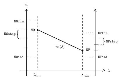
N0ini, N0fin, N0step, NFini, NFfin, NFstep refer to the initial estimative of the refractive index (see figure below). The initial estimates of the refractive index are the strictly decreasing linear functions which values vary between N0ini and N0fin with step N0step at LAMBDAmin and between NFini and NFfin with step NFstep at LAMBDAmax. So, the strictly decreasing linear functions used as initial estimates of are the linear functions which pass through the pairs:

(LAMBDAmin,N0), (LAMBDAmax,NF)

with

N0 = N0ini + u * N0step, u = 0, 1, 2, ...
NF = NFini + v * NFstep, v = 0, 1, 2, ...
N0 in [N0ini,N0fin], NF in [NFini,NFfin], and N0 > NF.

$Refractive Index initial guess$

An a priori knowledge of the refractive index of the material is needed to set these parameters.
K0ini, K0fin, K0step refer to the initial estimates of the attenuation coefficient (see figure below). In this case, we used a piecewise linear function, the values of which are K0 at LAMBDAmin, 0.1*K0 at LAMBDAmin+0.2*(LAMBDAmax-LAMBDAmin) and *K0 at LAMBDAmax, where K0 takes on the values

K0 = K0ini + z * K0step,z = 0, 1, 2, ...

inside the interval [K0ini,K0fin].

$Refractive Index initial guess$

Remark: Parameters described in 18 and 19 are meaningful only if you want to perform an initial estimative (when you set INIT=0); otherwise, they must be omitted. For systems with two or more films, if INIT=0 then parameters described from 12 to 19 must be repeated for each film. For systems with two or more films, if INIT=9 then parameters described from 12 to 17 must be repeated for each film.

One-film system example

As explained above, you can call PUMA either performing an initial estimative or using a previous estimate as initial guess, calling PUMA one, two, three or more times, as long as you find it necessary. This fact, combined with some clever choice of the input parameters in the sequence of calls, gives PUMA a good degree of flexibility.

Because, most of the time, it is enough to make three calls, we recommend, as a default procedure, to perform three calls, as follows.

In the first trial, chose an interval for the trial thicknesses around some value. Set the thickness step. Choose the attenuation coefficient inflection point interval to be the same of the spectrum interval.
Narrow the trial thicknesses interval around the previous retrieved thickness. Decrease the thickness step. Do the same for the attenuation coefficient inflection point. Increase the maximum number of iterations.
Fix the thickness as the previous retrieved thickness. Do the same for the inflection point. Once again, increase the maximum number of iterations.

As an example, suppose we have the gedanken film A of [1] (to reproduce this example in your computer, copy the input data file sigl0097t-dat.txt in the same directory where PUMA was installed). The trial sequence is as follows.

First Call

For the first trial, we have

puma sigl0097t 4 2 10 T 100 0540 1530 3000 1e+100 0 0010 0200 10 0540 1530 100 3 5 1 3 5 1 0.10 0.10 0.05

In this statement, we used

FNAME: sigl0097t. This film was generated using gedanken constants and simulates an a a-Si:H thin film deposited on a glass substrate with thickness of 97nm (see the file sigl0097t-dat.txt).
NLAYERS: 4 (first air layer + 1 film + substrate + last air layer)
SLAYER: 2 (the first air layer is called layer 0, the film is layer 1, the substrate is layer 2 and the last air layer is layer 3)
SUBSTRATE: 10 (Corning 7059 glass).
DATATYPE: T (transmittance).
NOBS: 100 (as recommended).
LAMBDAmin: 540 and LAMBDAmax: 1530. Note that the in the input file, the smallest wavelength is 1 and the greatest one is 5000.
MAXIT: 3000
QUAD: 1e+100
INIT: 0. That means we are running the initial estimative.
THICKNESSmin: 10, THICKNESSmax: 200 and THICKNESSstep: 10
INFLEmin: 540 , INFLEmax: 1530 and INFLEstep: 100
N0ini: 3, N0fin: 5, N0step: 1, NFini: 3, NFfin: 5, NFstep: 1
K0ini: 0.10, K0fin: 0.10, K0step: 0.05

You can see the first output file sigl0097t-inf.txt or the terminal output during this run. The retrieved thickness was 100nm, the retrieved attenuation coefficient inflection point was 540nm and the retrievals of the refractive index and the attenuation coefficient at the end of this run, were

Retrieval at the
end of the first PUMA call

Second Call

Once the first trial is finished, you can go to the second trial. If you look at the output file sigl0097t-inf.txt of the first call, you can see that the retrieved thickness was 100nm, the retrieved inflection point was 540nm and the quadratic error was 6.342857e-03. This last value may vary slightly from machine to machine, so do not expect to reproduce it exactly. With this at hand, we can go to the second trial:

puma sigl0097t 4 2 10 T 100 0540 1530 5000 6.342857e-03 9 0050 0150 01 0540 0540 100

where the bold font means which parameters were changed from the first call. Their meanings are

We increased the number of iterations from 3000 to 5000.
We made QUAD="previous quadratic error"= 6.342857e-03. This means that only thicknesses and constant estimations with a quadratic error smaller than this one will be saved.
As we are using the previously estimated optical constants to guide this new trial, we must set INIT=9.
For the new thickness interval, we choose the one centered at 100 (obtained previously), with +/- 50 of amplitude. Also, we decreased the step to 1.
As the retrieved value for the inflection point is considered good, we fixed it at 540 by making INFLEmin = INFLEmax = 540. In this case the INFLEstep is not considered at all and it can take any value).
The remaining parameters N0ini, N0fin, N0step,NFini, NFfin, NFstep, K0ini, K0fin, and K0step (which were only needed at the first call) must be omitted.

You can see the second output file sigl0097t-inf.txt or the terminal output during this run. The retrieved thickness was 97nm and the retrievals of the refractive index and the attenuation coefficient at the end of this run, were

Retrieval at
the end of the second PUMA call

Third Call

Finally, you can go to the third and last trial. If you look at the output file sigl0097t-inf.txt of the second call, you can see that the retrieved thickness is 97nm and the best quadratic error decreased to 1.773782e-04 (remember that the inflection point was fixed at 540nm). With this at hand, you can go the third and last trial:

puma sigl0097t 4 2 10 T 100 0540 1530 50000 1.773782e-04 9 0097 0097 01 0540 0540 100

where the bold font means, as before, which parameters were changed from the previous call. Their meanings are

We increased the number of iterations from 5000 to 50000.
We made QUAD="previous quadratic error"= 1.773782e-04. This means that only thicknesses and constant estimations with a quadratic error smaller than this one will be saved.
We considered the thickness as retrieved, with value 97nm. So we fix it by making THICKNESSmin = THICKNESSmax = 97. In this case the THICKNESSstep is not considered at all and it can take any value).

You can see the last output file sigl0097t-inf.txt or the terminal output during this run. The retrievals of refractive index and the attenuation coefficient at the end of this run, were

Retrieval at the
end of the third PUMA call

Two-films system example

As a second example, suppose we have the gedanken film AgB of [7] (to reproduce this example in your computer, copy the input data file AgB01000600t-dat.txt in the same directory where PUMA was installed). The trial sequence is as follows. Before running the parallel version of PUMA do not forget to start up your MPI Grid.

First Call

First of all, copy the executable file puma-par and the data file AgB01000600t-dat.txt to all the nodes of your MPI Grid.

For the first trial, submit to your MPI Grid, the following:

puma-par AgB01000600t 5 2 10 T 100 631 1621 5000 1e+100 0 50 150 10 631 631 1 3.5 4.5 0.5 3 4 0.5 0.5 0.5 1 550 650 10 631 631 1 3.5 4.5 0.5 3 4 0.5 0.5 0.5 1

In this statement, we used

FNAME: AgB01000600t. This film was generated using gedanken constants and simulates an a-Si:H thin film with tickness of 100nm deposited on one side of a glass substrate and an a-Si:H thin film with thickness of 600nm deposited on the other side of the glass substrate (see the file AgB01000600t-dat.txt).
NLAYERS: 5 (first air layer + film A + substrate + film B + last air layer)
SLAYER: 2 (the first air layer is called layer 0, the first film is layer 1, the substrate is layer 2, the second film is layer 3 and the last air layer is layer 4).
SUBSTRATE: 10 (Corning 7059 glass).
DATATYPE: T (transmittance).
NOBS: 100 (as recommended).
LAMBDAmin: 631 and LAMBDAmax: 1621.
MAXIT: 5000
QUAD: 1e+100
INIT: 0. That means we are running the initial estimative.

Parameters related to the first film (Film A):

THICKNESSmin: 50, THICKNESSmax: 150 and THICKNESSstep: 10
INFLEmin: 631 , INFLEmax: 631 and INFLEstep: 1
N0ini: 3.5, N0fin: 4.5, N0step: 0.5, NFini: 3, NFfin: 4, NFstep: 0.5
K0ini: 0.50, K0fin: 0.50, K0step: 1

Parameters related to the second film (Film B):

THICKNESSmin: 550, THICKNESSmax: 650 and THICKNESSstep: 10
INFLEmin: 631 , INFLEmax: 631 and INFLEstep: 1
N0ini: 3.5, N0fin: 4.5, N0step: 0.5, NFini: 3, NFfin: 4, NFstep: 0.5
K0ini: 0.50, K0fin: 0.50, K0step: 1

You can see the first output file AgB01000600t-inf.txt or the terminal output during this run (note that because of the nondeterministic order of execution of the subproblems, your output lines may be in a different order). The retrieved thicknesses were 100nm and 600nm for the first and the second film, respectively; while the retrievals of the refractive indexes and the attenuation coefficients at the end of this run, were

Retrieval at the
end of the first PUMA call

Second Call

First of all, copy file AgB01000600t-sol.txt (generated by the previous call to PUMA) to all the nodes of your MPI Grid.

Once the first trial is finished, we can go to the second trial. If you look at the output file AgB01000600t-inf.txt of the first call, you can see that the retrieved thicknesses were 100nm and 600nm for the first and the second film, respectively; while the quadratic error was 3.744793e-04. This last value may vary slightly from machine to machine, so do not expect to reproduce it exactly. With this at hand, we can go to the second trial.

For the second trial, submit to your MPI Grid, the following:

puma-par AgB01000600t 5 2 10 T 100 631 1621 100000 3.744793e-04 9 50 150 1 631 631 1 550 650 1 631 631 1

where the bold font means which parameters were changed from the first call. Their meanings are

We increased the number of iterations from 5000 to 100000.
We made QUAD="previous quadratic error"= 3.744793e-04. This means that only thicknesses and constant estimations with a quadratic error smaller than this one will be saved.
As we are using the previously estimated optical constants to guide this new trial, we must set INIT=9.
For the new thicknesses intervals, we choose the ones centered at the previously obtained values, with +/- 50 of amplitude (no changes from last run). Also, we decreased the step to 1.
The remaining parameters (for both films) N0ini, N0fin, N0step,NFini, NFfin, NFstep, K0ini, K0fin, and K0step (which were needed at the first call) must be omitted.

You can see the second output file AgB01000600t-inf.txt or the terminal output during this run (note that because of the nondeterministic order of execution of the subproblems, your output lines may be in a different order). The retrieved thicknesses were 100nm and 600nm for the first and the second film, respectively; the retrievals of the refractive indexes and the attenuation coefficients at the end of this run, were

Retrieval at the
end of the first PUMA call

Third Call

First of all, copy file AgB01000600t-sol.txt (generated by the previous call to PUMA) to all the nodes of your MPI Grid.

Finally, we can go to the third and last trial. If you look at the output file AgB01000600t-inf.txt of the second call, you can see that the retrieved thicknesses are 100nm and 600nm for the first and the second film, respectively; the best quadratic error decreased to 3.800786e-05. With this at hand, you can go the third and last trial.

For the third trial, submit to your MPI Grid, the following:

puma-par AgB01000600t 5 2 10 T 100 631 1621 1000000 3.800786e-05 9 100 100 1 631 631 1 600 600 1 631 631 1

where the bold font means, as before, which parameters were changed from the previous call. Their meanings are

We increased the number of iterations from 100000 to 1000000.
We made QUAD="previous quadratic error"= 3.800786e-05. This means that only thicknesses and constant estimations with a quadratic error smaller than this one will be saved.
We considered the thicknesses as retrieved, with values 100nm and 600nm for the first and the second film, respectively. So we fix it by making THICKNESSmin = THICKNESSmax = 100, for the first film, and THICKNESSmin = THICKNESSmax = 600, for the second film. In this case, the THICKNESSstep is not considered at all and it can take any value.

You can see the third output file AgB01000600t-inf.txt3 or the terminal output during this run. The retrievals of the refractive indexes and the attenuation coefficients at the end of this run, were

Retrieval at the
end of the first PUMA call

Remarks

The transmission T of the thin absorbing film deposited on a thick transparent substrate must be a rate stated as a proportion of one (something between zero and one) and not a percentage (between zero and one hundred).

The transmission formula being used assumes that the substrate is perfectly transparent. As a consequence of this limitation, the useful spectral ranges 350-2000nm for glass, 1250-2600nm for crystalline silicon, 200-1500nm for crystalline quartz, 360-800nm for glass slides and 300-2600nm for borosilicate substrates must be retained in the numerical experiments.

Everything we did in the examples above for transmittance, can be repeated for reflectance data and for both data (where both means to use transmittance and reflectance simultaneously). The analogous input files to the ones used in the one-film system example are sigl0097r-dat.txt (for reflectance data) and sigl0097b-dat.txt (for transmittance and reflectance data).

Related publications

E. G. Birgin, I. Chambouleyron, and J. M. Martínez, Estimation of optical constants of thin films using unconstrained optimization, Journal of Computational Physics 151, pp. 862-880, 1999.
[pdf] [ps]
The problem of estimating the thickness and the optical constants of thin films using transmission data only is very challenging from the mathematical point of view, and has a technological and an economic importance. In many cases it represents a very ill-conditioned inverse problem with many local-nonglobal solutions. In a recent publication we proposed nonlinear programming models for solving this problem.Well-known software for linearly constrained optimization was used with success for this purpose. In this paper we introduce an unconstrained formulation of the nonlinear programming model and we solve the estimation problem using a method based on repeated calls to a recently introduced unconstrained minimization algorithm. Numerical experiments on computer-generated films show that the new procedure is reliable.
M. Mulato, I. Chambouleyron, E. G. Birgin and J. M. Martínez, Determination of thickness and optical constants of a-Si:H films from transmittance data, Applied Physics Letters 77, pp. 2133-2135, 2000.
[pdf] [ps]
This work presents the first application of a recently developed numerical method to determine the thickness and the optical constants of thin films using experimental transmittance data only. The new method may be applied to films not displaying a fringe pattern and is shown to work for a-Si:H layers as thin as 100 nm. The performance and limitations of the method are discussed on the basis of experiments performed on a series of six a-Si:H samples grown under identical conditions, but with thickness varying from 98 nm to 1.2 mu m.
I. Chambouleyron, S. D. Ventura, E. G. Birgin, and J. M. Martínez, Optical constants and thickness determination of very thin amorphous semiconductor films, Journal of Applied Physics 92, pp. 3093-3102, 2002.
[pdf] [ps]
This contribution addresses the relevant question of retrieving, from transmittance data, the optical constants and thickness of very thin semiconductor and dielectric films. The retrieval process looks for a thickness that, subject to the physical input of the problem, minimizes the difference between the measured and the theoretical spectra. This is a highly underdetermined problem but, the use of approximate - though simple - functional dependences of the index of refraction and of the absorption coefficient on photon energy, used as an a priori information, allows surmounting the ill-posedness of the problem. The method is illustrated with the analysis of transmittance data of very thin amorphous silicon films. The method allows retrieving physically meaningful solutions for films as thin as 300 A. The estimated parameters agree well with known data or with optical parameters measured by independent methods. The limitations of the adopted model and the shortcomings of the optimization algorithm are presented and discussed.
E. G. Birgin, I. Chambouleyron, and J. M. Martínez, Optimization problems in the estimation of parameters of thin films and the elimination of the influence of the substrate, Journal of Computational and Applied Mathematics 152, pp. 35-50, 2003.
[pdf] [ps]
In a recent paper, the authors introduced a method to estimate optical parameters of thin films using transmission data. The associated model assumes that the film is deposited on a completely transparent substrate. It has been observed, however, that small absorption of substrates affect in a nonnegligible way the transmitted energy. The question arises of the reliability of the estimation method to retrieve optical parameters in the presence of substrates of different thicknesses and absorption degrees. In this paper, transmission spectra of thin films deposited on non-transparent substrates are generated and, as a first approximation, the method based on transparent substrates is used to estimate the optical parameters. As expected, the method is good when the absorption of the substrate is very small, but fails when one deals with less transparent substrates. To overcome this drawback, an iterative procedure is introduced, that allows one to approximate the transmittance with transparent substrate, given the transmittance with absorbent substrate. The updated method turns out to be almost as efficient in the case of absorbent substrates as it was in the case of transparent ones.
E. G. Birgin, I. Chambouleyron, J. M. Martínez, and S. D. Ventura, Estimation of optical parameters of very thin films, Applied Numerical Mathematics 47, pp. 109-119, 2003.
[pdf] [ps]
In recent papers, the problem of estimating the thickness and the optical constants (refractive index and absorption coefficient) of thin films using only transmittance data has been addressed by means of optimization techniques. Models were proposed for solving this problem using linearly constrained optimization and unconstrained optimization. However, the optical parameters of "very thin" films could not be recovered with methods that are successful in other situations. Here we introduce an optimization technique that seems to be efficient for recovering the parameters of very thin films.
S. Ventura, E. G. Birgin, J. M. Martínez and I. Chambouleyron, Optimization techniques for the estimation of the thickness and the optical parameters of thin films using reflectance data, Journal of Applied Physics 97, 043512, 2005.
[pdf] [ps]
The present work considers the problem of estimating the thickness and the optical constants (extinction coefficient and refractive index) of thin films from the spectrum of normal reflectance R. This is an ill-conditioned highly underdetermined inverse problem. The estimation is done in the spectral range where the film is not opaque. The idea behind the choice of this particular spectral range is to compare the film characteristics retrieved from transmittance T and from reflectance data. In the first part of the paper a compact formula for R is deduced. The approach to deconvolute the R data is to use well known information on the dependence of the optical constants on photon energy of semiconductors and dielectrics and to formulate the estimation as a nonlinear optimization problem. Previous publications of the group on the subject provide the guidelines for designing the new procedures. The consistency of the approach is tested with computer generated thin films and also with measured R and T spectral data of an a-Si:H film deposited onto glass. The algorithms can handle satisfactorily the problem of a poor photometric accuracy in reflectance data, as well as a partial linearity of the detector response.
R. Andrade, E. G. Birgin, I. Chambouleyron, J. M. Martínez and S. D. Ventura, Estimation of the thickness and the optical parameters of several superimposed thin films using optimization, Applied Optics 47, pp. 5208-5220, 2008.
[pdf] [ps]
The Reverse Engineering problem addressed in the present research consists in estimating the thicknesses and the optical parameters of two thin films deposited on a transparent substrate using only transmittance data through the whole stack. To the present author's knowledge this is the first report on the retrieval of the optical constants and the thickness of multiple film structures using transmittance data only. The same methodology may be used if the available data correspond to normal reflectance. The software used in this work is freely available through the PUMA Project web page (http://www.ime.usp.br/~egbirgin/puma/).

Last updated at January 13, 2009

*Full Name:
*E-mail
*Institution:
*Type:
Description of your problem (optional):
	I agree with the conditions-of-use above.

* Required!

Sequential version (recommended for one-film systems)

Parallel version (recommended for systems with two or more films)

First Call

Second Call

Third Call

First Call

Second Call

Third Call