Algorithms and their analysis
A pedagogical introduction
V.W.Setzer & F.H. Carvalheiro
Dept. of Computer Science, University of São Paulo
www.ime.usp.br/~vwsetzer
Translation from [1] by VWS, English revision by C.M.Tolman
– Version 1.4, March 14, 2009
1. Introduction
Algorithms have existed since ancient times. The execution of a sum of 2 numbers with many digits follows an algorithm; the well known "Euclid Algorithm" for the calculation of a maximal common divisor, if its author may be assumed to be its discoverer, dates to the 3rd century BC.
Today, the notion and domain of algorithms has become absolutely essential, because every "working" computer program, that is, producing the expected results, is probably a description of an algorithm. (If the reader finds the "probably" a bit strange, he or she probably needs to better understand what algorithms are and what programs are...) Furthermore, if one wishes to develop a program for a computer, the correct way of doing it would be to initially look for the most adequate method for the solution to a problem, specifying this solution as an algorithm and, afterwards, expressing it in some computer language for its insertion into the computer, followed by its (automatic) interpretation or translation into machine language, and its execution.
From an educational point of view, it seems to us essential that one teaches that "programming a computer" does not mean giving the machine some commands expressed in the syntax of some programming language, modifying and then rearranging them until the expected result is obtained, as happens with an electronic (video) game. The essence of programming and computing, the subject that should really attract students’ interest to that area, is the development and analysis of algorithms.
This paper presents a teaching activity based upon the notion of algorithms and their complexity analysis. According to our experience, we consider it to be adequate to the senior high school classes. Its duration is approximately 3 hours. It does not require previous computing experience from students. It employs some physical pedagogical material, presenting a problem with numbers in the form of a competitive manual game. The students solve the problem in groups, having a reasonable space for exercising their creativity. Afterwards they compare the different solutions obtained by different groups. In the sequel, the instructor makes an abstraction of the concepts involved in the solution of the proposed problem, and presents a more complex and efficient solution. Then he or she introduces advanced concepts such as algorithm correctness and complexity, the notion of an optimal algorithm and the intractability of certain problems. All this is done without any connection to a computer, so the availability of such machines is not necessary for introducing conceptual notions of computing and programming. On the other hand, if computers are available, our method may serve for the introduction of practical programming.
2. The proposed problem
For introducing the desired ideas we have chosen the problem of sorting n numbers.
2.1. Statement
As a pedagogical didactic, the instructor tells the students that his manager gave him the following problem:
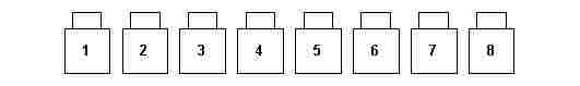
"Here is a board with pockets numbered from 1 to 8 (fig. 1). Inside each pocket there is a strip of card upon which a natural number is written. You are supposed to rearrange the strips such that they are in increasing order from left to right, according to the following rules:
R1. It is possible to lift up a strip from its compartment, in order to examine its contents, that is, the number written upon it.
fig. 1
R2. If a strip is inside a pocket, with its number hidden, it is considered to be unknown. You are not supposed to memorise the contents of the pockets.
R3. At most 2 strips may be lifted at the same time (fig. 2).
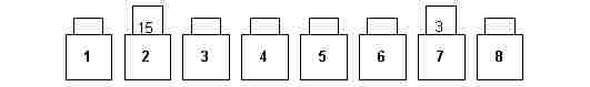
fig. 2
R4. The contents of 2 lifted strips may be compared, determining which one contains the smaller number.
R5. Two strips may be exchanged between their pockets. (fig. 3 in relation to fig. 2).
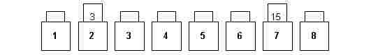
fig. 3
I am going to take advantage of the fact that you are here to count on your help (suppose I could not solve the problem), in groups of up to 3 participants. Let us see which 3 groups solve the problem first; as a magnificent prize they will receive the boards they used with their respective strips."
2.2 Practical considerations
We have used white paper boards of approximately 80 cm x 25 cm; the pockets are made of coloured paper board about 9 cm x 9 cm, with a stapled bottom side and glued on their left and right sides. Strips are made of another colour, measuring 5 cm x 12 cm, with the numbers (up to 3 digits) written on their hidden part. A board may be folded in two to facilitate transportation and storage.
Another possibility, less illustrative but much simpler, is using 8 pieces of paper of the same color and size, set in a line over the desk. In the sequel, we will use the description with the paper board and pockets.
The instructor states the problem, hands out a sheet of paper with the rules, explains them using a board and then distributes one board to each group. In general it takes from 10 to 15 minutes for the first 3 groups to come out with a solution to the problem.
3. Obtained solutions
3.1. Description and generalisation of the solutions
The instructor tells the participants that his manager is going to give him further tasks, so there may be additional boards with any number of pockets. Then he asks the participants of each winning group for their help, describing the method they used, so that he may learn it. He also asks them for a generalisation to any given number n of pockets. He asks the other participants to remain silent, paying attention to verify that their solution was the same.
The instructor must help the groups to describe in a reasonably logical way the processes they figured out. One of the most common problems is to give a condition to determine that the sorting process has reached an end. After the descriptions of the winning groups, the instructor asks if any other group has a different idea, and asks for a description.
3.2. Types of solution
In general, participants come out with the 3 most simple and traditional solutions for the sorting problem, described in any introductory text on algorithms [2]. When 2 winning groups reached the same solution, in general some non-winning group reached the remaining third solution.
The instructor shows that the 3 methods are described in the literature, and exhibits the corresponding chapters in text books. This makes the students highly impressed, because they become conscious of their ability to invent processes that are internationally described. He asks for the name that they would give their methods and presents the traditional names used in the literature. Hand-outs are distributed showing each one of the methods with an example. For the orientation of readers that are not familiar with Computer Science, we present these methods in the sequel; the distributed sheets contain exactly the same words as presented below. Notice the progressive evolution of the algorithm formalisation. Version 1 shows the description as usually given by participants. In the next versions we progressively approach a formal algorithm. After the following sections we make some practical observations.
3.2.1. The selection method
We will call the contents of the pockets C1, ...,Cn.
Version 1 (informal description). Compare C1 with C2 and exchange their strips if C1 > C2. Then do the same with C1 and C3, then with C1 and C4, etc. up to C1 and Cn. At the end of this phase the smallest element of the sequence will be in pocket 1. Now we perform a second phase, comparing C2 and C3, exchanging them if C2 > C3, then doing the same for C2 and C4, C2 and C5, ..., C2 and Cn. After this, pocket 2 will contain the second smallest element of the sequence. We repeat these phases beginning with C3 then with C4, up to Cn-1. The strips will then be ordered as desired.
Version 2 (initial formalisation)
for i varying from 1 up to n-1
do: compare Ci with Ci+1, then with Ci+2, ... , up to Ci with Cn, exchanging each pair of strips if Ci > Ci+j.
Version 3 (final formalisation)
for i varying from 1 up to n-1
do: for j varying from i+1 to n
do: if Ci > Cj exchange the contents of the pockets
Example (the table shows the situation after the execution of the step indicated by the values of i and j):
|
i |
j |
pocket: |
1 |
2 |
3 |
4 |
5 |
6 |
7 |
8 |
|
|
|
initial value: |
5 |
10 |
3 |
7 |
15 |
2 |
1 |
9 |
|
1 |
2 |
|
5 |
10 |
3 |
7 |
15 |
2 |
1 |
9 |
|
|
3 |
|
3 |
10 |
5 |
7 |
15 |
2 |
1 |
9 |
|
... |
||||||||||
|
|
6 |
|
2 |
10 |
5 |
7 |
15 |
3 |
1 |
9 |
|
|
7 |
|
1 |
10 |
5 |
7 |
15 |
3 |
2 |
9 |
|
|
8 |
|
1 |
10 |
5 |
7 |
15 |
3 |
2 |
9 |
|
2 |
3 |
|
1 |
5 |
10 |
7 |
15 |
3 |
2 |
9 |
|
... |
||||||||||
|
|
8 |
|
1 |
2 |
10 |
7 |
15 |
5 |
3 |
9 |
|
3 |
4 |
|
1 |
2 |
7 |
10 |
15 |
5 |
3 |
9 |
|
... |
||||||||||
|
|
8 |
|
1 |
2 |
3 |
10 |
15 |
7 |
5 |
9 |
|
4 |
5 |
|
1 |
2 |
3 |
10 |
15 |
7 |
5 |
9 |
|
... |
||||||||||
|
|
8 |
|
1 |
2 |
3 |
5 |
15 |
10 |
7 |
9 |
|
5 |
6 |
|
1 |
2 |
3 |
5 |
10 |
15 |
7 |
9 |
|
... |
||||||||||
|
|
8 |
|
1 |
2 |
3 |
5 |
7 |
15 |
10 |
9 |
|
6 |
7 |
|
1 |
2 |
3 |
5 |
7 |
10 |
15 |
9 |
|
|
8 |
|
1 |
2 |
3 |
5 |
7 |
9 |
15 |
10 |
|
7 |
8 |
|
1 |
2 |
3 |
5 |
7 |
9 |
10 |
15 |
Version 1 (informal description). Compare C1 with C2 and exchange their contents if C1 > C2. Then do the same with C2 and C3, then with C3 and C4, until Cn-1 and Cn. At the end of this phase the greatest element of the sequence will be in pocket n. Now we proceed to a second phase, making comparisons up to Cn-1, obtaining the 2nd greatest element of the sequence in pocket n-1. We repeat these phases making comparisons up to Cn-2, then Cn-3, .. and, at last, C2. The strips will then be sorted.
Version 2 (initial formalisation)
for i varying from n down to 2
do: compare C1 with C2, C2 with C3, ... , up to Ci-1 with Ci, exchanging each pair of strips in their pockets if Cj > Cj+1
Version 3 (final formalisation)
for i varying from n down to
do: for j varying from 1 up to i-1
do: if Cj > Cj+1, exchange their strips
|
i |
j |
pocket: |
1 |
2 |
3 |
4 |
5 |
6 |
7 |
8 |
|
|
|
initial value: |
5 |
10 |
3 |
7 |
15 |
2 |
1 |
9 |
|
8 |
1 |
|
5 |
10 |
3 |
7 |
15 |
2 |
1 |
9 |
|
|
2 |
|
5 |
3 |
10 |
7 |
15 |
2 |
1 |
9 |
|
|
3 |
|
5 |
3 |
7 |
10 |
15 |
2 |
1 |
9 |
|
|
4 |
|
5 |
3 |
7 |
10 |
15 |
2 |
1 |
9 |
|
|
5 |
|
5 |
3 |
7 |
10 |
2 |
15 |
1 |
9 |
|
|
6 |
|
5 |
3 |
7 |
10 |
2 |
1 |
15 |
9 |
|
|
7 |
|
5 |
3 |
7 |
10 |
2 |
1 |
9 |
15 |
|
7 |
1 |
|
3 |
5 |
7 |
10 |
2 |
1 |
9 |
15 |
|
... |
||||||||||
|
|
6 |
|
3 |
5 |
7 |
2 |
1 |
9 |
10 |
15 |
|
6 |
1 |
|
3 |
5 |
7 |
2 |
1 |
9 |
10 |
15 |
|
... |
||||||||||
|
|
5 |
|
3 |
5 |
2 |
1 |
7 |
9 |
10 |
15 |
|
5 |
1 |
|
3 |
5 |
2 |
1 |
7 |
9 |
10 |
15 |
|
... |
||||||||||
|
|
4 |
|
3 |
2 |
1 |
5 |
7 |
9 |
10 |
15 |
|
4 |
1 |
|
2 |
3 |
1 |
5 |
7 |
9 |
10 |
15 |
|
... |
||||||||||
|
|
3 |
|
2 |
1 |
3 |
5 |
7 |
9 |
10 |
15 |
|
3 |
1 |
|
1 |
2 |
3 |
5 |
7 |
9 |
10 |
15 |
|
|
2 |
|
1 |
2 |
3 |
5 |
7 |
9 |
10 |
15 |
|
2 |
1 |
|
1 |
2 |
3 |
5 |
7 |
9 |
10 |
15 |
Version 1 (informal description). In an initial phase, compare C2 with C1 and exchange their strips if C2 < C1. After this we can guarantee that the sequence of C1 and C2 is in ascending order. In the second phase, compare C3 with C2, exchanging their strips if C3 < C2. If there was an exchange, compare C2 with C1, exchanging their strips if C2 < C1. After this 2nd phase, we guarantee that the sequence from C1 up to C3 is sorted. We repeat these phases beginning with C4 then with C5, until Cn. The last phase (which begins with Cn) works like this: compare Cn with Cn-1 and exchange their strips if Cn < Cn-1; if there was an exchange, compare Cn-1 with Cn-2 and exchange their strips if Cn-1 < Cn-2; repeat this process until it is not necessary to exchange the contents of an adjacent pair of pockets, or reaching the comparison and eventual exchange of C1 with C2.
Version 2 (initial formalisation)
for i varying from 2 to n
do: compare successively the elements of pairs (Cj , Cj-1) for j from i down to 2 or until we find Cj > Cj-1;
for each pair of this collection, exchange Cj with Cj-1 if Cj < Cj-1
Version 3 (final formalisation)
for i varying from 2 to n
do: j ← i;
while (Cj < Cj-1)
and (j > 1)
do: exchange Cj
and Cj-1; j ← j-1
|
i |
j |
pocket: |
1 |
2 |
3 |
4 |
5 |
6 |
7 |
8 |
|
|
|
initial value: |
5 |
10 |
3 |
7 |
15 |
2 |
1 |
9 |
|
2 |
2 |
|
|
|
|
|
|
|
|
|
|
3 |
3 |
|
5 |
3 |
10 |
7 |
15 |
2 |
1 |
9 |
|
|
2 |
|
3 |
5 |
10 |
7 |
15 |
2 |
1 |
9 |
|
4 |
4 |
|
3 |
5 |
7 |
10 |
15 |
2 |
1 |
9 |
|
|
3 |
|
|
|
|
|
|
|
|
|
|
5 |
5 |
|
|
|
|
|
|
|
|
|
|
6 |
6 |
|
3 |
5 |
7 |
10 |
2 |
15 |
1 |
9 |
|
|
5 |
|
3 |
5 |
7 |
2 |
10 |
15 |
1 |
9 |
|
|
4 |
|
3 |
5 |
2 |
7 |
10 |
15 |
1 |
9 |
|
|
3 |
|
3 |
2 |
5 |
7 |
10 |
15 |
1 |
9 |
|
|
2 |
|
2 |
3 |
5 |
7 |
10 |
15 |
1 |
9 |
|
7 |
7 |
|
2 |
3 |
5 |
7 |
10 |
1 |
15 |
9 |
|
|
6 |
|
2 |
3 |
5 |
7 |
1 |
10 |
15 |
9 |
|
|
5 |
|
2 |
3 |
5 |
1 |
7 |
10 |
15 |
9 |
|
|
4 |
|
2 |
3 |
1 |
5 |
7 |
10 |
15 |
9 |
|
|
3 |
|
2 |
1 |
3 |
5 |
7 |
10 |
15 |
9 |
|
|
2 |
|
1 |
2 |
3 |
5 |
7 |
10 |
15 |
9 |
|
8 |
8 |
|
1 |
2 |
3 |
5 |
7 |
10 |
9 |
15 |
|
|
7 |
|
1 |
2 |
3 |
5 |
7 |
9 |
10 |
15 |
|
|
6 |
|
|
|
|
|
|
|
|
|
A variation of the selection method covered by the instructor (and already suggested by a group) is to perform just one exchange in each run of comparisons from i to n; for this one could simply leave the strip in pocket j lifted up, with the smaller number encountered from i to j, i ≤ j ≤ n; later if a strip is found with a smaller number, we lift the latter up and pull down the former; the smaller is finally exchanged with the i-th strip. In spite of the fact that we maintained the number of comparisons, the single exchange diminishes the number of operations. This is a beginning of the introduction of the idea of efficiency.
An improvement of the bubble method, which has many times been pointed out by participants, is to stop the execution of the process just after a phase with no exchange, because in this case the sequence is already sorted.
4. Analysing the solutions
The instructor continues telling his life’s drama: after presenting the various solutions to his manager, the latter will certainly ask him which one is best. He awaits some help from the participants, guiding them with questions like: "What does it mean to be the best?"; "How can we compare the different efficiencies?"; "What operations require more work to be executed?".
The instructor ends up suggesting (or confirming some suggestion from one of the participants) that a good measure is to count in each case the number of comparisons and exchanges.
Analysing the 3 methods, it is possible to see that in the selection and bubble methods there are always (n-1) + (n-2) + ... + 1 = n(n-1)/2 comparisons. In the insertion method, if the sequence is initially sorted, there are n-1 comparisons, but in the worst case there may also be n(n-1)/2 comparisons. The same occurs with the improved bubble method, as described in section 3.3. As for the number of exchanges, in the worst case, the selection method with the improvement described in section 3.3 executes n-1 exchanges (one per phase), while the other methods execute n(n-1)/2 exchanges (one for each comparison, if the strips are initially in reverse order).
The instructor informs the participants that he is very unlucky, and that his manager knows it. His manager will therefore want to know what is the efficiency in the worst case. As we saw, in this situation the 3 methods perform the same number of comparisons, but the selection method has some advantage because it performs less exchanges.
From these considerations, the notion of complexity is introduced. In the described cases, it is of the order of n2, written O(n2), as one may observe by the calculated number of comparisons. It is shown that this means for big values of n that other terms with smaller degree than 2 may be disregarded. It follows that doubling the number of elements to be sorted quadruples the time for the whole sort.
5. A more efficient method
Attention: I have written a new chapter 5, with a much simpler and illustrative method. VWS.
5.1. Motivation
The instructor relates that his manager will probably say: "Your friends took 30-40 minutes to reach these solutions. If they would work for a whole morning, would they come up with a more efficient solution?". He asks the participants what they think about this question. In general, most of them think it is possible to obtain a better method, but there are always some that think no better method can exist.
A more efficient method is then introduced, tree sort, which uses exactly the same rules R1 to R5, with the following additions:
R6. The use of additional pockets is permitted; they follow the rules R1 to R5.
R7. It is possible to erase the number of a strip and write another one in its place.
5.2. Tree sort
The method is presented on the blackboard as follows:
i) 8 numbers are written side by side (fig. 4).
![]()
fig 4
It is observed that in the previous methods one made a scan comparing pairs of strips, just to keep one single piece of information: what is the smallest (or greatest) number of the sequence. Another possibility would be to make just one scan, but storing more information. It would be better still if in each comparison we could keep the result in an extra pocket (or more precisely, copy the result into an extra pocket), for example the smaller number.
ii) In a first phase compare the 8 initial numbers, two at a time, resulting in a sequence (or level) of auxiliary pockets (fig. 5).
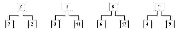
fig. 5
Observe that if we wish to find the smallest number of the sequence, it suffices to look for it among the numbers at this new level.
iii) In a subsequent phase, we compare the resulting 4 numbers of this level, two by two, resulting in a 3rd level of auxiliary pockets.
iv) Repeat these phases until a level with just one pocket is obtained (fig. 6).
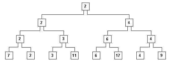
fig. 6
v) The structure that appears in fig. 6 is called a tree. Each pocket is called a node. The uppermost node is called the root and the lowest nodes are called the leaves (the tree is upside down – this is the usual way computer scientists regard the world after they have used their computers too intensively…). The other nodes are called intermediary nodes. A node x is the parent of node y (its child), if x is in the level immediately above y, and is connected to y. Notice that in fig. 6 each non-leaf node is the parent of exactly 2 children. These children nodes are called sibling nodes in relationship to each other. We may generalise the definition of the parent and child nodes to be ascendant and descendent nodes.
vi) Observe that the smallest number is the root (2 in fig. 6), because for each non-leaf node the following property P is valid: its contents are less than or equal to any of its descendants. The root contains the first element of the ordered sequence.
vii) Now we erase this number from the root node, and from all nodes where it appears (this is called a hierarchical path from the root down to a leaf), creating empty nodes (those having no number. fig. 7)
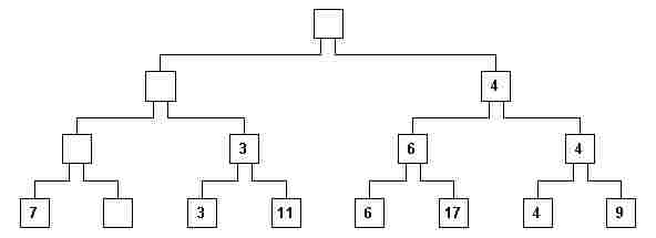
fig. 7
It is interesting to note that game rules R1 - R5 continue to be valid: it suffices to lift up a strip of a parent node and of one of its children to decide which one has the same value as its parent.
viii) Now the tree has to be rearranged. Only the erased nodes have to be reconstituted, because they don’t satisfy rule P anymore. The contents of empty nodes should not be used in the comparisons. Beginning with the empty leaf node, we see that its sibling (7 in fig. 7) should be moved to its parent node. (fig. 8).
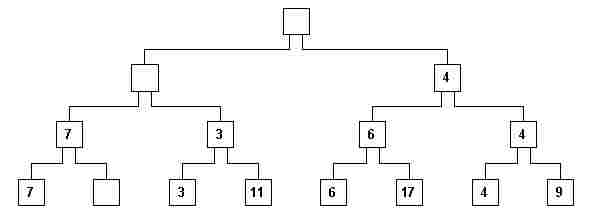
fig. 8
ix) It would be interesting to preserve the comparison technique, because dealing with "empty" seems rather strange. For this we may ask the participants: what number would you insert into the empty leaf node, such that its sibling node (7 in the example) would always be smaller? Participants always answer correctly: infinity! It is commented that in computers there is never an "infinity"; in general we choose the greatest possible number which may be inserted into a "strip" (storage word in a computer). On the blackboard we insert the infinity sign ¥ into every node that was empty (fig 9).
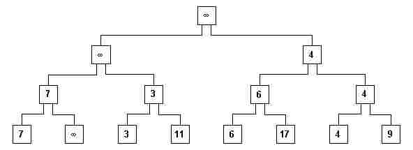
fig. 9
x) The reconstruction of the tree is done along the hierarchical path up to the root, which will then contain the next element of the ordered sequence (fig. 10).
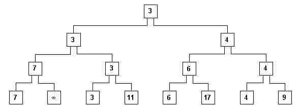
fig. 10
xi) The new root is eliminated, replacing the corresponding elements of the hierarchical path with ¥ (fig. 11).
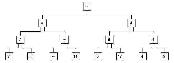
fig. 11
xii) The process is repeated until all n numbers have been erased from the root.
5.3. Analysis
Let’s continue counting the number of comparisons.
To construct the initial full tree (fig. 6) the number of comparisons was exactly the number of auxiliary pockets that were created. If there are n leaves, at the level of their parents there will be n/2 pockets, then at the level of their parents n/4, etc. down to 1.
In general, participants observe at this point that n cannot be an arbitrary number, suggesting that it has to be an even number. We observe then that if n is not a power of 2, it is possible to complete the leaf nodes with additional ones containing ¥ , until the number of leaves is the next power of 2. The total number of comparisons is, then, for an n which is a power of 2,
C = 1 + 2 + 4 + ... + n/4 + n/2
We have the sum of a geometric progression with rate q = 2; the sum C of a GP is given by:
C = a1 (qk - 1) / (q - 1) (1)
where a1 is the first term, and k the number of terms (if students haven’t had geometrical progressions in their course, this would be a nice occasion to deduce this formula; but then additional time or classes should be alloted.). How many terms do we have in our case? As many as the number of levels in auxiliary pockets.
Inspecting fig.6, we can see that the root level 0 has 1 element, level 1 has 2, level 2 has 22, level 3 has 23, ..., thus j (the leaf level) has 2j elements. But we know that 2j = n . Thus, j = log2n (height of the tree). As we are looking for the number of levels from 0 to j-1, we have k = j . Thus k = log2n . Replacing in (1):
C = 1 (2log2 n - 1) / (2 - 1) = n - 1
Therefore, n - 1 comparisons have to be made to build the tree.
Replacing the root node, and every one with the same number by ¥ , takes log2n (height of the tree) comparisons on the "way down". After this it is necessary to get the sibling of the last (leaf) node where an ¥ was inserted, and perform the comparisons until the root is reached, reconstituting the tree. We have log2n additional comparisons in this "ascent". Thus, for each root value there are 2log2n comparisons. As the first root was deduced in a special manner, and the last does not have to be eliminated, we have (n-1)2log2n comparisons in these "ascents" and "descents". Then, the total number of comparisons is:
n - 1 + 2(n-1)log2n
Which gives us a complexity of O(nlog2n), much better than the 3 initial methods, which had O(n2). This is shown in the next table, with the number of comparisons in each case. Participants become very impressed with the order of magnitude O(n2) methods, and the fact that tree sort, albeit being more complex, has so much advantage. Note that 2048 elements is a very small number compared to the number of students in a university or the number of names in a telephone book, for example.
It is also interesting to observe that "tree sort" should not be used in every case, because as shown in the table, up to n = 16, the other methods are more efficient.
Next the total number of pockets is calculated: n leaves plus n-1 auxiliary pockets, plus n to keep the elements of the ordered sequence. This gives 3n-1, that is, this method uses 3 times as many pockets as the initial 3 methods. It is then mentioned that it is possible to use exactly the same auxiliary pockets, obtaining the so-called "heap sort" [2].
|
n |
n(n-1)/2 |
(n-1)+2(n-1)log2n |
Column 2 compared with Column 3 |
|
1 |
0 |
0 |
= |
|
2 |
1 |
3 |
67% better |
|
4 |
6 |
15 |
60% better |
|
8 |
28 |
49 |
43% better |
|
16 |
120 |
135 |
12% better |
|
32 |
496 |
341 |
1.4 times worse |
|
64 |
2016 |
819 |
2.5 times worse |
|
128 |
8128 |
1905 |
4.3 times worse |
|
256 |
32640 |
4335 |
7.5 times worse |
|
512 |
130816 |
9709 |
13.5 times worse |
|
1024 |
523776 |
21483 |
24.4 times worse |
|
2048 |
2096128 |
47081 |
44.5 times worse |
6. The notion of an optimal algorithm
The instructor, referring again to his manager, reminds the participants that the latter is very demanding, and asks what his manager is going to ask next.
In general, the participants formulate the correct question: is there any better sorting method?
The instructor says that it is possible to formally prove that there is no sort algorithm based upon comparisons of the elements of the sequence, having complexity smaller than nlog2n. He gives an indication of how this fact may be demonstrated, employing the "tree sort" tree of comparisons: one cannot perform less the comparisons than shown in the algorithm. He calls attention to the fact that it is impossible to find a sort algorithm (based upon comparisons) linear on time as a function of the number of elements to be ordered. For example, if sorting 1000 numbers takes 1 second, 2000 numbers will certainly take more than 2 seconds. This is a fact that the majority of professionals working in data processing do not know (this statement is based upon the experience of the first author posing this question to the data processing professionals who were taking one of the hundreds of lectures and courses he had already given).
This notion of the optimal algorithm is quite useful to illustrate the importance of Computing Theory, in particular Algorithmic Analysis. Most professionals, if not all of them, become satisfied when they find an algorithm which solves a problem, without questioning if there is a better algorithm and its "distance" from the theoretical optimum. Unfortunately, computers have become very cheap and fast, so if an algorithm is badly chosen and designed, and the machine is taking to long to give the expected solutions, one just buys a more powerful, faster one.
If the instructor’s manager had asked for a linear sorting algorithm using comparisons, knowledge of the theory would permit the instructor to dismiss his task without having lost his job for not accomplishing it.
The problem of optimal sort has been solved, but there exist other open problems, which are the subject of research in the area of algorithmic analysis. Research is done both in order to obtain better algorithms, as well as to demonstrate optimal complexities, that is, of the non-existence of better algorithms if the optimal has already been reached.
The travelling salesman problem for example, namely finding the path that a person has to take to visit cities with a minimal cost for the trip, is still open as far as finding an algorithm with polynomial complexity: every currently known algorithm has exponential complexity.
7. Computational Questions
Using the sort examples, it is possible to introduce fundamental concepts of Computer Science. For example, what does a professional working in this area do when he encounters a problem? He looks for algorithms; we need to then find what characterises an algorithm. Next, he tries to formally describe the algorithm found and program it. He has to demonstrate that the algorithm is correct, and analyse it regarding its complexity, verifying that it is tractable with respect to the time taken for processing.
7.1. What is an algorithm
An algorithm is a finite sequence of elementary steps, each one containing a well-defined mathematical operation. The execution of the sequence should terminate for any given set of input data. Notice that this is a characterisation and not a formal definition (because it may be impossible to prove that execution terminates).
7.2. The difficulty of obtaining a formal description, programming
The sort problem has used the following steps for the solution of a problem: 1) Solution of a particular problem (sorting 8 numbers); 2) Generalisation (sorting an arbitrary number of numbers); 3) Formal description of the generalised method (necessary for subsequent analysis and programming for the further introduction into a computer).
The difficulty of formally describing a solution method for a certain problem became clear when the winning groups tried to formulate it.
It is shown that, having a good description, programming it for a computer is a trivial task. Listings of PASCAL programs which implement the 3 sort methods described in section 3.2. are handed out (See Appendix). Each statement is briefly described.
7.3. Correctness of an algorithm
The proof of the correctness of an algorithm consists in demonstrating that it correctly executes the desired process, that is, that it reaches the desired solution. There are formal methods for proving correctness using Mathematical Logic. In this area there are two classes of problems: proof of correct execution; and proof that execution terminates for any input. This last question is called the halting problem.
Another technique consists of mathematically specifying a problem, then transforming this specification using formal rules (which should have previously been demonstrated to be correct), until one reaches an algorithm which may be formulated in a programming language. This area is called Program Development by (Formal) Transformations. Instead of proving that the program is correct, it is deduced in a correct way (one of the big problems with proving a program correct is that when it is not correct, in most of the cases nothing can be concluded).
7.4. Problems with correct or incorrect solutions
Consider the following problem: There are n cities which must be connected by train. The cost of constructing each section connecting a pair of cities is known (fig. 12). Some connections are not feasible (there are lakes, mountains, etc.) and are not represented. The problem is to find a unique connexed net (that is, making it possible to travel from any one city to any other) such that it may be built with the least total construction cost.
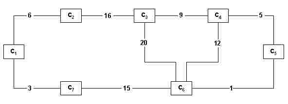
fig. 12
Kruskal (see for example [3]) proposed in 1956 an algorithm which is classified under the generic name of Greedy Algorithms. Initially, the sections are sorted in ascending cost order (an application for the sort algorithms...). For the case of fig. 12, we get the following sequence (note that in this example there are no two sections with the same cost, so the cost identifies the section):
1 3 5 6 7 9 12 15 16 20
Next, this ordered sequence is scanned, and in each step a section connecting two cities as yet unconnected by some path is inserted into the defined sequence. Thus the steps are:
a) 1; b) 1 3; c) 1 3 5; d) 1 3 5 6; e) 1 3 5 6 9; f) 1 3 5 6 9 15
Note that in the transition from step (d) to step (e) the section with cost 7 was ignored, because it connected two cities which were already indirectly connected by the section with costs 3 and 6. Note also that during this process one may have various disconnected subnets; for example, after pass (b) we already have this situation, which remains so up to the last step, when the two disconnected subnets are connected.
The resulting net has the form of a tree (in the example, with root 1 and hierarchical paths 1-5-9 and 1-15-3-6), called a minimal spanning tree [3]. Kruskal proved that it really had a minimum cost, thus solving the problem.
It is interesting to discuss a little with the participants the optimality of the solution: for example, when choosing the next section, isn’t it possible to force the future choice of more expensive and undesirable sections? It is mentioned that the proof of optimality is not trivial and is the subject of a field of Computer Science called Graph Theory. It is essential to insist on the importance of proving the correctness of an algorithm, and that for our own example that it really deduces the optimal solution. It is an example that formalisation is essential to verify some intuitive certainty or doubt.
The name "greedy method" comes from the fact that in each step the best alternative is chosen. Nevertheless, it is not a method that leads to the optimal solution for any problem. For example, suppose a zoologist breeds various animals: lions, tigers, elephants, zebras, giraffes, etc. He has a certain profit for each animal that he sells. He receives an order for a certain number of animals, irrespective of the species. The problem is to organise just one trip to carry the mix of animals that give the highest total profit. Unfortunately, it is not possible to transport certain animals at the same time (his truck has no compartments): for example, lions are incompatible with zebras – not all of the latter would reach the destination intact...
In this case the greedy method does not provide an optimal solution. For example, suppose the profit for a lion is 20 and for a zebra is 2. There is just one lion but 11 zebras. The greedy method would initially choose the lion, but all the zebras together would give a greater profit.
The generic problem is to find what is called the maximal independent set. For the optimal solution of this problem, it is not known if there exists a polynomial complexity algorithm for the execution time. Existing algorithms use combinations of elements of the various sets, resulting in a factorial complexity (which is worse than exponential, because the multiplying factor increases by 1 at each new multiplication). In the next section we give an example of this complexity, showing how disastrous it is.
7.5. Problems with inefficient solutions
A simple example of the problem with an inherently inefficient solution is the following. A company has designed a new hand calculator with a display and calculation resolution of 8 digits. It wishes to test it in order to verify that each calculator is working perfectly. A brilliant technician decides to construct an apparatus to make these exhaustive tests.
In the case of additions, the test apparatus introduces 2 terms, and verifies the obtained result with the expected correct result. Suppose the apparatus has the capacity of testing 1 million additions per second (this speed is much higher than the capacity of hand calculators, because if they execute one calculation every tenth of a second they have a speed more than satisfactory for their purpose). How long will it take to test all possible additions? There are 108 possible different numbers in each term, therefore 1016 possible combinations of values for the two terms. This would mean 1010 seconds to perform all the tests. Assuming 10000 seconds per hour (instead of 3600) we have 106 hours of tests; assuming 25 hours per day, we have 4.104 days; assuming 400 days per year we have a total (underestimated) of 100 years. That is, the problem is totally intractable using this method. (Note that this proves that hand calculators are not exhaustively tested... It is a marvel of electronic engineering that with just a few tests it is possible to conclude the "correctness" of the whole machine.)
In general, game simulation problems are of this nature: it is necessary to test many combinations (the possible moves in each situation). This makes them sometimes impossible to treat using computers, unless strategies for the elimination of many combinations are applied. This is a subject covered by the algorithm area (wrongly) called "Artificial Intelligence". It is interesting to note that these algorithms have very little to do with our way of playing the corresponding games. In fact, a Grand Master in chess cannot know and describe the intuition process that makes him guess the best move for each situation.
8. Results
Through the described activities, an introduction is made to a wide area of fundamental concepts of the Theory of Computation. As it has been shown, this introduction begins with a physical manipulation by the participants, thus avoiding an excessively abstract teaching method that has no connection to the students’ reality. A computer screen cannot replace students’ physical activity, because the latter may deal with real, and not abstract, objects. Furthermore, our proposal involves a social aspect through the formation of groups, who may not only discuss in the realm of ideas, but also may "do with their hands". A purely abstract level is reached later, but is related to the physical experience. In this sense we have here an example of "bottom-up" learning, which seems to us much more adequate. The concrete example precedes abstraction; when the latter is reached, students will not consider it as something absolutely strange, outside of their experience.
Our experience has shown that physical activities stimulate creativity. In fact, participants have been stating that they would never have found the sort of algorithms they did if they had not manipulated the card strips. During the practical activities students encounter some previously studied mathematical concepts: summation of number progressions, logarithms and their properties, combinatorics. In two of the assessments written by participants just after the class, the following phrases were found:
"This activity is valid mainly for those who have no idea why they are learning Mathematics at school. Through the given concrete examples, it is possible to understand why there is so much theory."
"I could better understand the fact that we are really going to use the Mathematics learned at school."
The pedagogical material and the game rules (see section 2) were designed so that the solutions found by participants could be expressed through algorithms and be close to a computer program. We believe it is essential that the idea students have of computers and computing be changed. The idea they currently have is a false one due to the use of electronic games, sophisticated text and graphic editors, etc., and the emotions associated with them. Students on our introductory Computer Science course invariably become frustrated with its conceptual form: they had other expectations. Thus the fact that the activities described here do not use a computer go in the direction of changing that false idea. One of the participants wrote: "The class showed me that taking a course in Computer Science does not mean using the computer the whole day."
When this paper was written, in 1993, 11 classes had been given, with a total of approximately 450 students. The great majority of them wrote, in their assessment, that they had no difficulties following the presented algorithms and their analysis.
There is a lot of hyperbole on the use of computers in schools. The first author has expressed his opinion that computers should only be used in the senior high school grade, when learning the practical uses of computers [6, 7]. Through another educational program that he organised, "The Computer Day", taking 8 hours [5], it was shown that, in general, students less than 17 years of age don’t have an interest in the conceptual and structural aspects of a computer: they only want to play wit it. Thus he recommends that the Activities described in this paper should be applied to that age, that is, to senior high school students. They may be preceded by an introduction to the internal logical structure of computers, through activities also developed by the first author: a theatre play simulating the internal functioning of a computer [8] and the learning and use of Machine Language of a very simple simulated computer [4]. We had the opportunity of showing here how new, important and wide concepts may be introduced in such a way that some fundamental aspects of computing become clear to students. Finally we consider that Mathematics is a proper subject for the activities described here. Computing, from the algorithmic point of view, is a Mathematical Science.
References
[1] Setzer, V.W & R.Hirata Jr. Algoritmos e sua análise: uma introdução didática. São Paulo: Caderno da Revista do Professor de Matemática, Brazilian Mathematical Society, Vol. 4, No. 1, 1993. pp. 1-38.
[2] Wirth, N. Algorithms and Data Structures. Englewood Cliffs: Prentice-Hall, 1986.
[3] Harel, D. Algorithmics – the Spirit of Computing. Reading: Addison-Wesley, 1987.
[4] Setzer, V.W & R.Hirata Jr. HIPO-PC: an educational software for introducing computers (in Portuguese). Technical Report RT-MAC-8809. São Paulo: Dept. of Computer Science, University of São Paulo (USP), 1989. Executable versions of the HIPO-PC simulator in English and Portuguese are available via e-mail through the first editor.
[5] Setzer, V.W & R.Hirata Jr. The Computer Day: a brief introduction to computers and computing (in Portuguese). Ciência e Cultura 42, 5/6 (May/June 1990), pp. 333-340, reprinted in the same publication as [1].
[6] Setzer, V.W. Computers in Education. Edinburgh: Floris Books, 1989. See also the enlarged edition in German, Computer in der Schule? Thesen und Argumente. Stuttgart: Verlag Freies Geistesleben, 1992.
[7] Setzer, V.W & L.W.Monke. An alternative view on computers in education: why, when, how. To be published in 2000 by Humpton Press as a chapter of a book edited by R. Muffoleto, also available at the first author’s web site.
[8] Setzer, V.W., "The ‘Paper Computer’ – a pedagogical activity for the introduction of basic concepts of computers", available at the first author’s web site (see address above).
APPENDIX
Programs in PASCAL
Program Selection;
{ Given N and a sequence of N numbers, sorts them in ascending order }
{ by the selection method. At the end, prints the ordered sequence. }
Var
N, { Number of elements in the sequence }
I, J: integer; { Indices }
C: array[1..100] of real; { The sequence has at most 100 elements }
Aux: real; { Auxiliary variable used in the exchange }
{ of the contents of 2 pockets. }
Begin
{ Input the sequence }
write(’Enter the size of the sequence, less than or equal to 100’);
readln(N);
for I:=1 to N
do begin
write(’Enter the next number of the sequence’);
readln(C[I])
end;
{ Sort }
for I:=1 to N-1
do for J:=I+1 to N
do if C[I] > C[J]
then begin { Exchange C[I] with C[J] }
Aux:=C[I];
C[I]:=C[J];
C[J]:=Aux
end;
{ Print }
writeln(’The ordered sequence is:’);
for I:=1 to N
do write(C[I],’ ’);
end.
Program Bubble;
{ Given N and a sequence of N numbers, sorts them in ascending order }
{ by the bubble method. At the end, prints the ordered sequence. }
Var
...
Begin
...
{ Sort }
for I:=N downto 2
do for J:=1 to I-1
do if C[J] > C[J+1]
then begin { Exchange C[J] with C[J+1] }
Aux:=C[J];
C[J]:=C[J+1];
C[J+1]:=Aux;
end;
...
end.
Program Insertion;
{ Given N and a sequence of N numbers, sorts them in ascending order }
{ by the insertion method. At the end, prints the ordered sequence. }
Var
...
Begin
...
{ Sort }
for I:=2 to N
do begin
J:=I;
while (C[J] < C[J-1]) and (J > 1)
do begin { Exchange C[J] with C[J-1] }
Aux:=C[J];
C[J]:=C[J-1];
C[J-1]:=Aux;
end;
end;
...
end.